First Model: Lessons from a 32% Baseline

Today marks a crucial milestone for the AstroSpectro project: the first end-to-end training run of our stellar type classification model. After setting up a robust acquisition and processing pipeline for 5000 spectra from the LAMOST DR5 survey, it was time to see what our first approach could achieve.

The First Iteration: A Simple but Honest Model​

To establish a baseline, the goal was to build the simplest possible model in order to validate the integrity of the processing chain. The strategy was as follows:

• Model : A RandomForestClassifier, a robust and well-understood algorithm.
• Features : Only four characteristics, based on the position of the best-known absorption lines Hα, Hβ, CaII H & K. The goal was to verify whether this minimal information already contained a predictive signal.

The Result: 32% Accuracy​

After training and evaluation on a test set of 1250 spectra, the model reached an overall accuracy of 32%.

Although this score may seem modest, it is an extremely promising starting point. In a classification problem with so many classes A, B, C, F, G, K, M, N, s, random prediction would only achieve about 9% correct answers. Our 32% score is therefore more than three times better than chance, which proves that our pipeline works and that the features, even simple ones, contain an exploitable signal.

Features used for training: ['feature_Hα', 'feature_Hβ', 'feature_CaIIK', 'feature_CaIIH']
Number of samples: 5000, Number of features: 4
Training the model on 3750 samples...

--- Evaluation Report ---

            precision    recall  f1-score   support

         A       0.40      0.59      0.48        79
         B       0.00      0.00      0.00         1
         C       0.00      0.00      0.00         1
         D       0.00      0.00      0.00         1
         F       0.41      0.51      0.46       239
         G       0.51      0.26      0.34       393
         K       0.37      0.24      0.29       294
         M       0.14      0.13      0.14       152
         N       0.30      0.37      0.33        89
         W       0.00      0.00      0.00         0
         s       0.00      0.00      0.00         1

  accuracy                           0.32      1250
 macro avg       0.19      0.19      0.18      1250
weighted avg     0.39      0.32      0.33      1250

But the most interesting part is not the score itself, but what the model's errors teach us.

The Analysis: The Confusion Matrix Speaks​

The confusion matrix is a true map of our model's "thinking". Two observations stand out immediately:

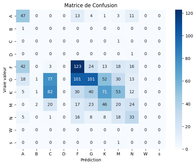
1. Data Imbalance: The model is unable to classify stars of type B, C, D or s, because it saw only a single example of each in the test set. This is a classic lesson in AI: a model cannot learn what it does not see.
2. "Physical Confusion": Where the model makes mistakes, it does so in a logical way. For example, it massively confuses G-type stars with F and K types. This is normal: these types are adjacent in the spectral sequence and look very similar. The model has therefore learned the stellar "geography" well, but struggles to draw precise boundaries.

The Root Cause: The Missing Features Problem​

Analysis of our extracted features revealed the heart of the problem. A graph showing the percentage of null values for each feature is quite clear:

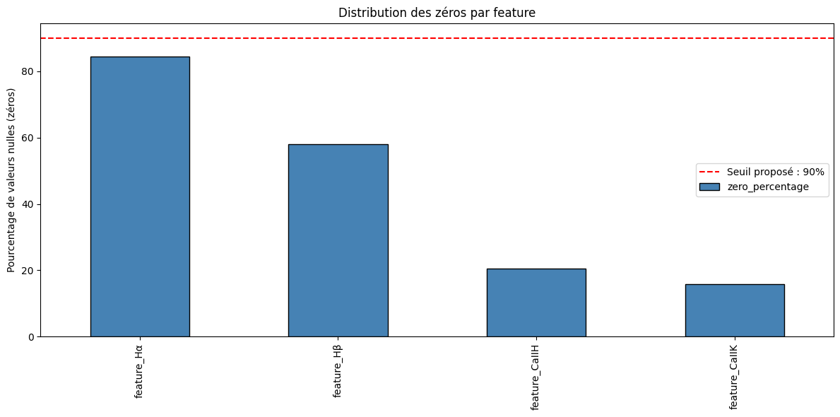
This graph, which analyzes our entire dataset of 5000 spectra, reveals a surprising reality: the feature based on the Hα line is absent in more than 80% of cases. The Hβ and CaII H/K lines are detected more frequently, but they still remain missing in a non-negligible fraction of the observations.

The model therefore had to make its decisions based on very incomplete information. Reaching 32% under these conditions proves that the calcium lines and Hβ are powerful indicators, but also that the model is strongly limited by the difficulty of extracting a clear Hα signal with the current parameters.

Next Steps: The Hunt for Real Features Is On!​

This first result is not an endpoint, but a documented starting point. The roadmap for the next iteration is clear: we need to provide our model with better-quality "ingredients".

1. Measure Strength, Not Presence: The next version of the pipeline will no longer only determine whether a line is present, but will measure its depth (through peak prominence). This is much richer physical information.
2. Create Ratio Features: We will compute ratios between the depths of different lines. These ratios are well-known temperature indicators in astrophysics and should help the model better distinguish adjacent classes (such as F, G and K).
3. Clean the Dataset: For the next evaluation, we will focus on the classes for which we have a sufficient number of examples A, F, G, K, M in order to obtain more reliable and interpretable performance metrics.

This 32% baseline is the foundation on which we will build. Every future improvement can be measured against this starting point, demonstrating the direct impact of our feature engineering work.

Stay tuned!