

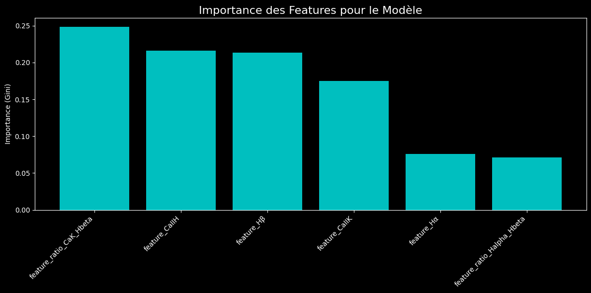
I built a pipeline that models spectral classification based on the principles of stellar physics. The model autonomously learned that Calcium and Hydrogen line-strength ratios are the best temperature indicators, validating our feature engineering approach and allowing us to reach 56% accuracy.
Today, after several iterations of debugging, analysis, and optimization, we reached a significant milestone, increasing the model accuracy from 32% to a very respectable 56%. Here is the story of that progression.
Iteration 1: From Line Presence to Line Strength
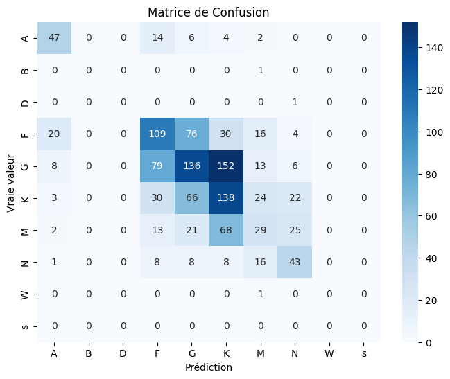
The first improvement consisted in moving from a binary feature (is the line present?) to a continuous measurement: the line strength, approximated by the "prominence" of the absorption peak. This change had an immediate impact, raising our overall accuracy from 32% to 40%. This step confirmed that the amount of physical information contained in the strength of a line is much richer than its mere presence.
View detailed results
Removal of overly rare classes: ['C']

Features used for training: ['feature_Hα', 'feature_Hβ', 'feature_CaIIK', 'feature_CaIIH']
Number of samples: 4999, Number of features: 4
> Training the model on 3749 samples...
> Model trained.

--- Evaluation Report ---
            precision    recall  f1-score   support

         A       0.58      0.64      0.61        73
         B       0.00      0.00      0.00         1
         D       0.00      0.00      0.00         1
         F       0.43      0.43      0.43       255
         G       0.43      0.35      0.38       394
         K       0.34      0.49      0.40       283
         M       0.28      0.18      0.22       158
         N       0.43      0.51      0.46        84
         W       0.00      0.00      0.00         1
         s       0.00      0.00      0.00         0

  accuracy                           0.40      1250
 macro avg       0.25      0.26      0.25      1250
weighted avg     0.40      0.40      0.40      1250
Iteration 2: The Power of Spectral Ratios
With a solid new baseline, we introduced even more sophisticated features: strength ratios between different lines. In astrophysics, these ratios are extremely powerful temperature indicators.
feature_ratio_CaK_Hbeta = CaII K / Hβfeature_ratio_Halpha_Hbeta = Hα / Hβ
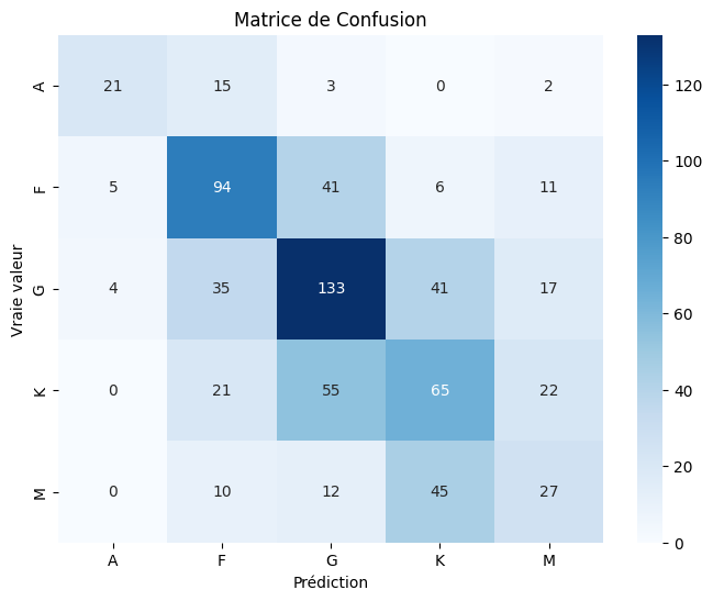
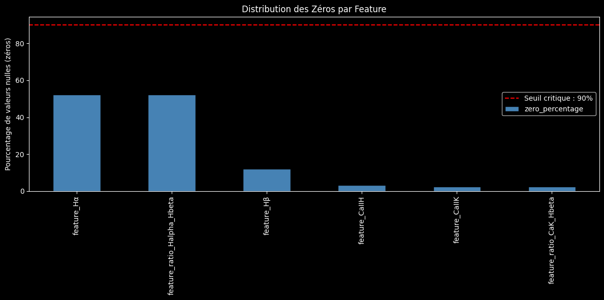
Adding just these two ratios once again pushed the model forward, reaching 50% accuracy. The confusion matrix showed a clear improvement, but a feature-quality analysis revealed a critical weakness: the Hα line was missing in more than 50% of the spectra, making the ratios unreliable.
View detailed results
--- Loading dataset: features_20250723T225208Z.csv ---
> 250 rows with invalid or null labels removed.
> Removal of overly rare classes: ['W', 'C', 'D', 'B', 's']

Features used: ['feature_Hα', 'feature_Hβ', 'feature_CaIIK', 'feature_CaIIH', 'feature_ratio_CaK_Hbeta', 'feature_ratio_Halpha_Hbeta']
Final number of samples: 2740, Number of features: 6

--- STEP 5: Model Training and Evaluation ---
> Training the model on 2055 samples...
> Model trained.

--- Evaluation Report ---
            precision    recall  f1-score   support

         A       0.70      0.51      0.59        41
         F       0.54      0.60      0.57       157
         G       0.55      0.58      0.56       230
         K       0.41      0.40      0.41       163
         M       0.34      0.29      0.31        94

  accuracy                           0.50       685
 macro avg       0.51      0.48      0.49       685
weighted avg     0.49      0.50      0.49       685
Final Iteration: Tuning Through Visualization
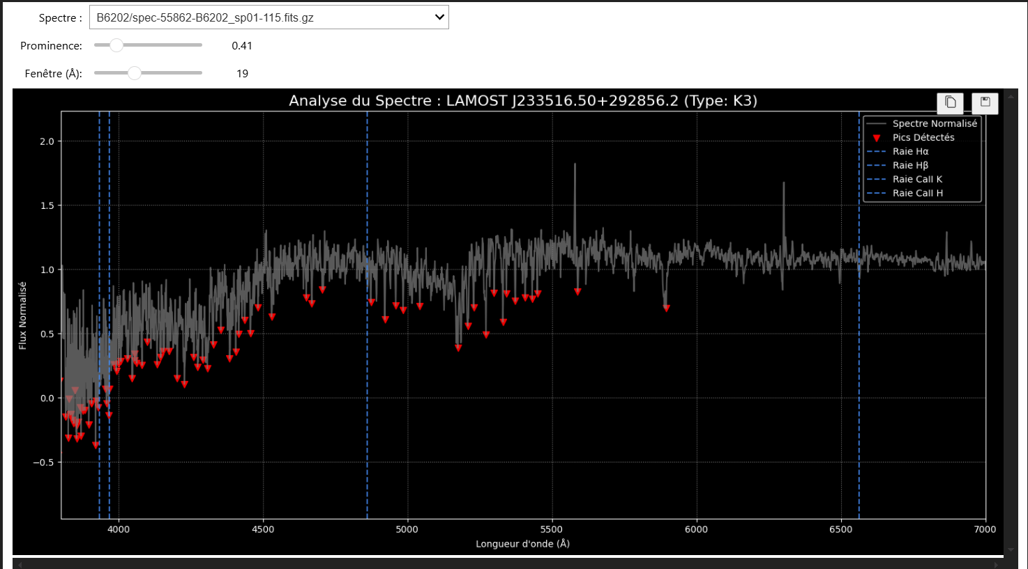
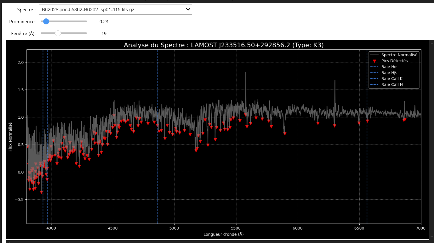
At this stage, our visualization tools became crucial. The analysis showed that our peak-detection parameter (prominence) was too strict and ignored many real but shallower lines.
Thanks to our interactive spectrum analyzer, we were able to tune this parameter in real time. An optimized value of prominence=0.23 was identified, allowing us to recover a large number of lines that had previously been ignored.
The Final Result: 56% Accuracy
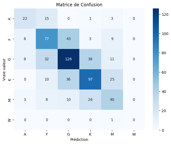
After rerunning the full pipeline with this optimized parameter on a new batch of 2607 spectra, the results exceeded our expectations:
- Overall Accuracy: 56%
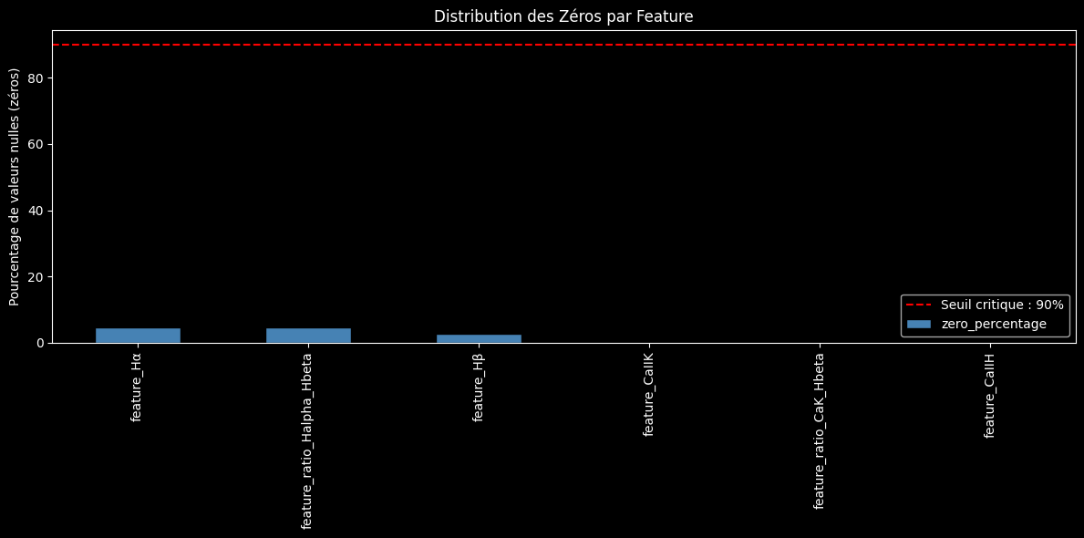
- Feature Quality: The missing-value problem was almost eliminated, with all base features present in more than 95% of cases.
- Feature Relevance: Feature importance is now much better balanced.
feature_Hβand theratio_CaK_Hbetastand out as the most powerful indicators, but all features now contribute meaningfully.
The final confusion matrix shows a much clearer diagonal, a sign of a more confident and more accurate model, with F1 scores above 0.54 for all main classes.
View detailed results
--- Loading dataset: features_20250724T012617Z.csv ---
> 383 rows with invalid or null labels removed.
> Removal of overly rare classes: ['s', 'B', 'D', 'C']

Features used: ['feature_Hα', 'feature_Hβ', 'feature_CaIIK', 'feature_CaIIH', 'feature_ratio_CaK_Hbeta', 'feature_ratio_Halpha_Hbeta']
Final number of samples: 2607, Number of features: 6

--- STEP 5: Model Training and Evaluation ---
> Training the model on 1955 samples...
> Model trained.

--- Evaluation Report ---
            precision    recall  f1-score   support

         A       0.54      0.54      0.54        41
         F       0.54      0.55      0.55       140
         G       0.59      0.59      0.59       215
         K       0.59      0.58      0.58       168
         M       0.45      0.46      0.45        87
         W       0.00      0.00      0.00         1

  accuracy                           0.56       652
 macro avg       0.45      0.45      0.45       652
weighted avg     0.55      0.56      0.56       652
Conclusion and Next Adventures
This research sprint was a striking demonstration of the power of the iterative method in data science. Starting from a simple model, and improving it step by step based on result analysis, we improved our baseline by 24 percentage points.
The AstroSpectro project now has a robust production pipeline and a suite of powerful analysis tools. The next exploration paths are already on the table:
- Enrich the features to better classify cool stars (type M) by adding molecular bands.
- Experiment with more powerful models such as XGBoost or neural networks.
- Move toward Deep Learning by using the full spectrum as input to a convolutional neural network (CNN).
The laboratory is built. The tools are sharpened. The adventure continues! 🚀