Attention & GradCAM
Grad-CAM (CNNs)
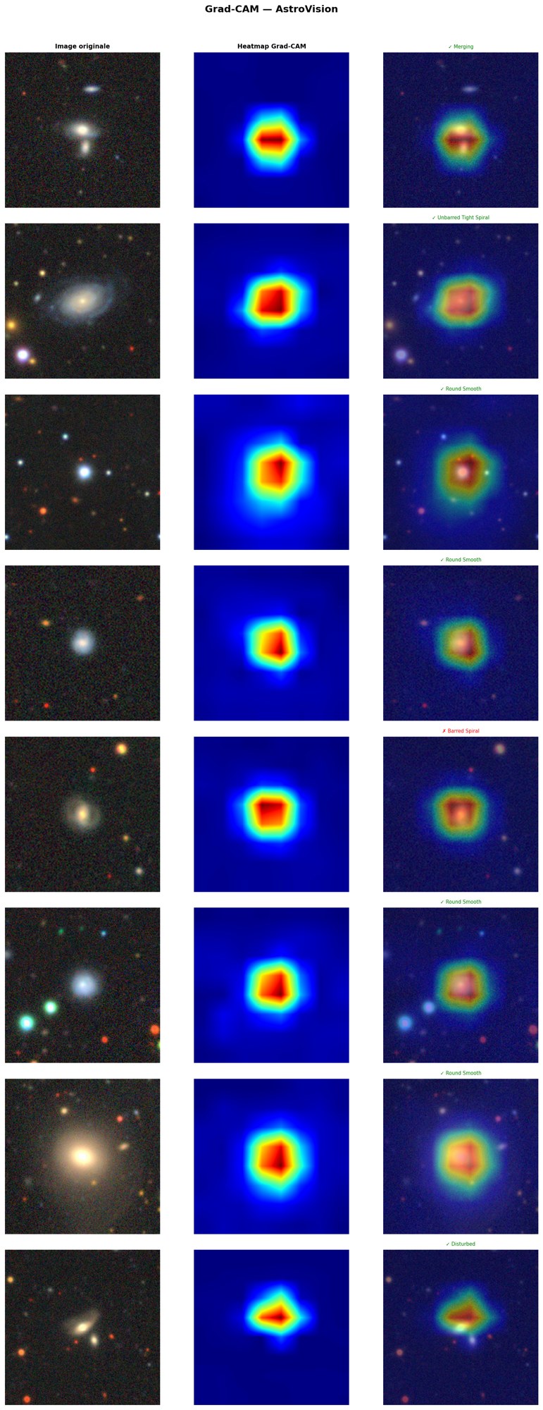
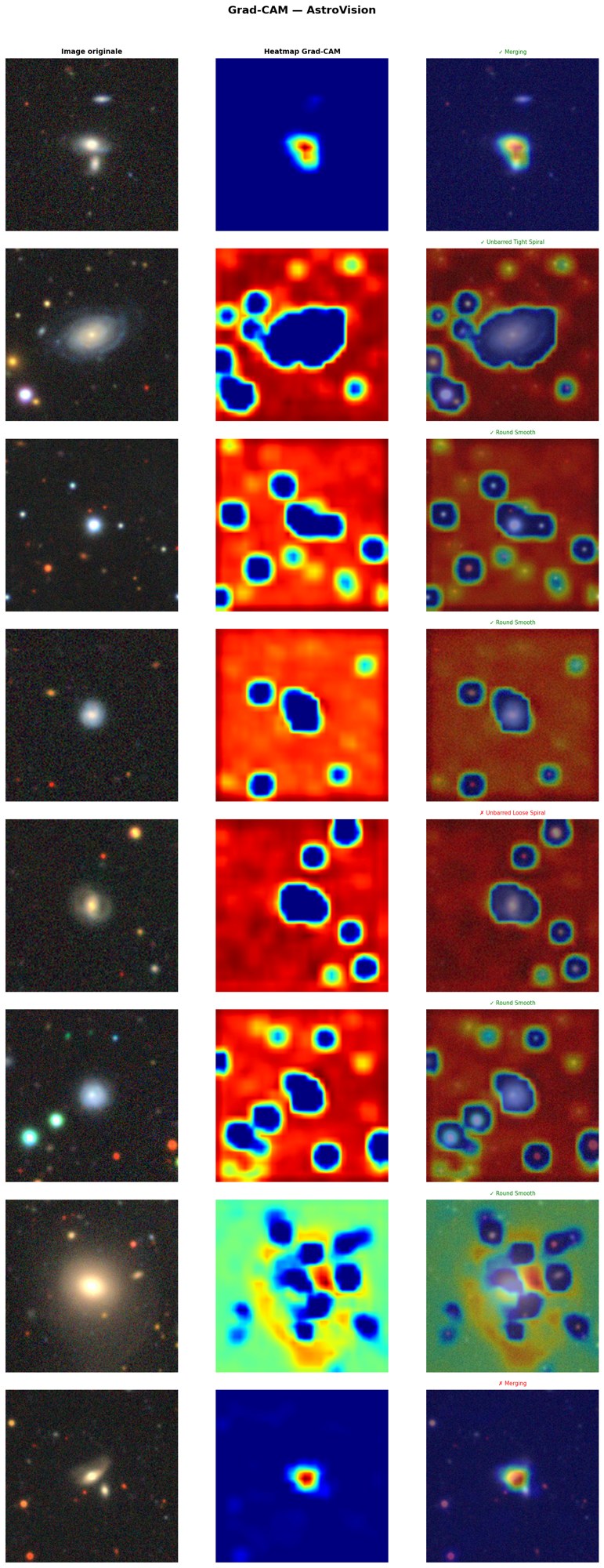
GradCAM hooks a target layer, weights its activations by the spatially averaged gradient of the class logit, applies a ReLU, upsamples to the input size and normalises to [0, 1]. Target layers: the 128→256 convolution for SimpleCNN, the last features block for EfficientNet-B0 (model.gradcam_target). plot_gradcam_grid renders image · heat map · overlay with the predicted class and a ✓ / ✗ marker.
A heat map shows where the logit is sensitive, not that the model uses a physically meaningful feature. The figures are qualitative; no quantitative faithfulness test (deletion curves, sanity checks) was run.
DINOv2 attention (ViT)
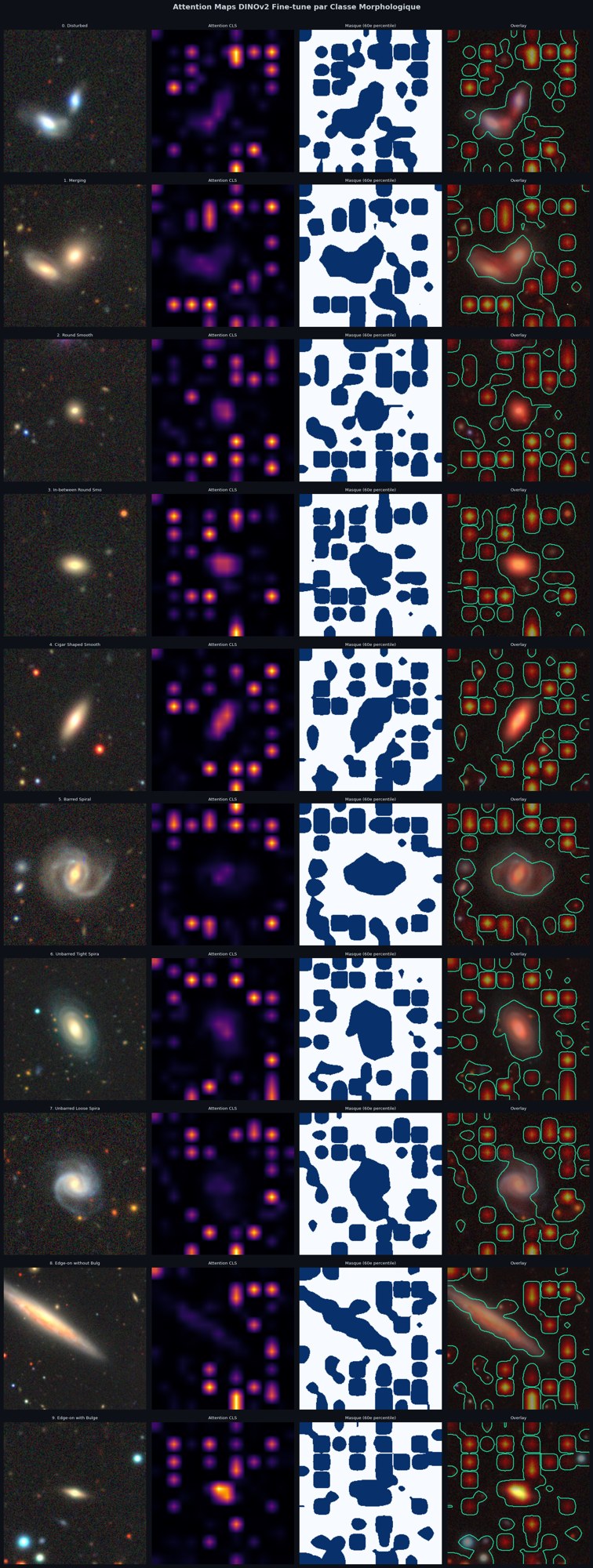
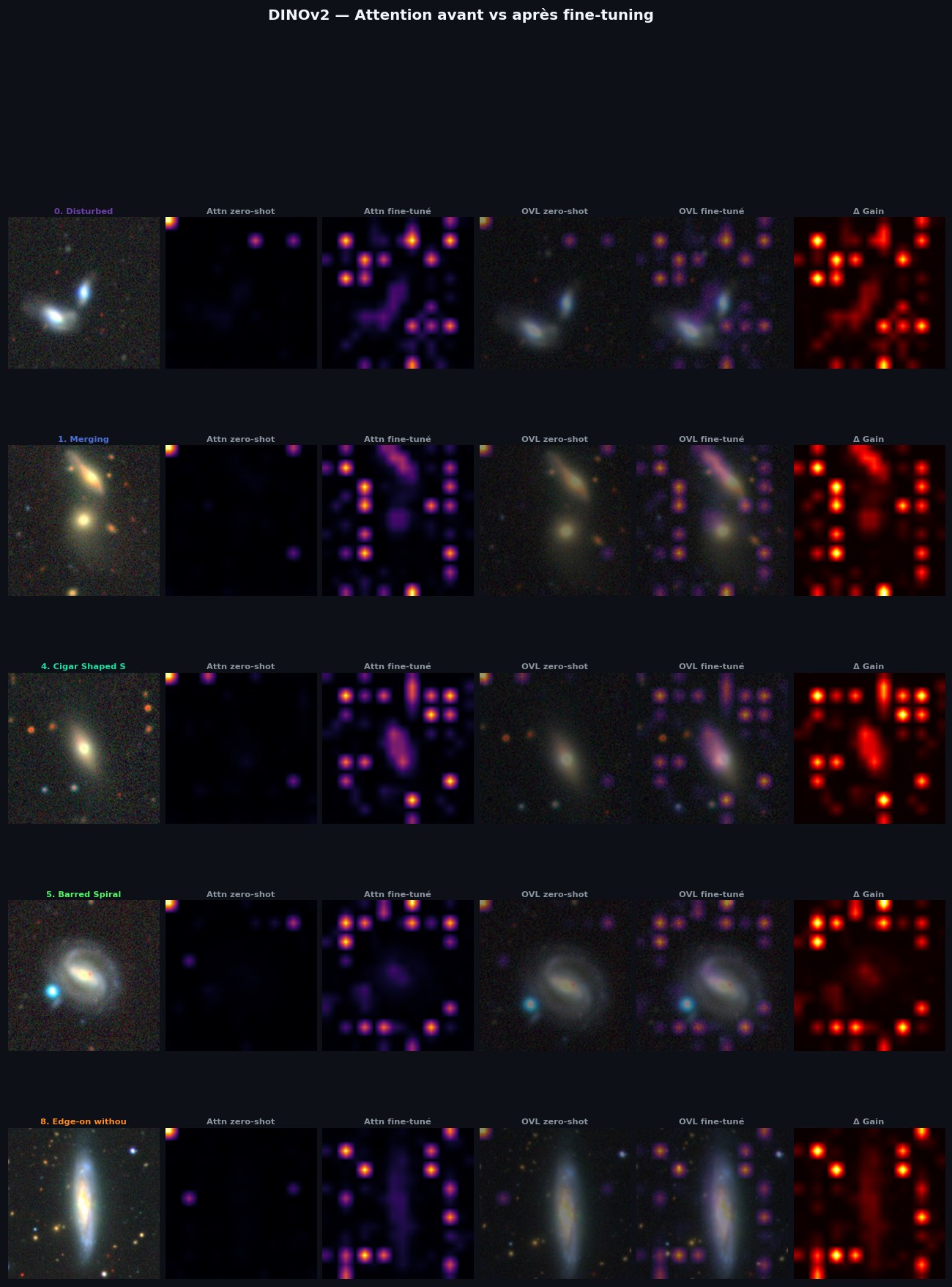
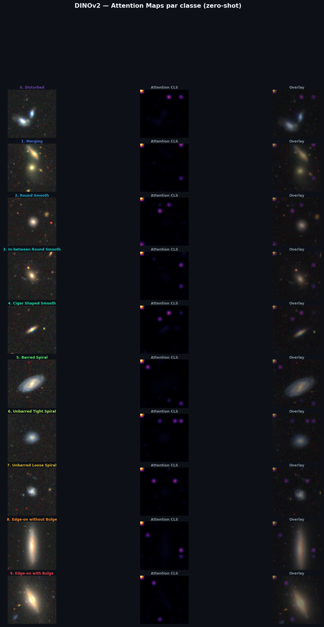
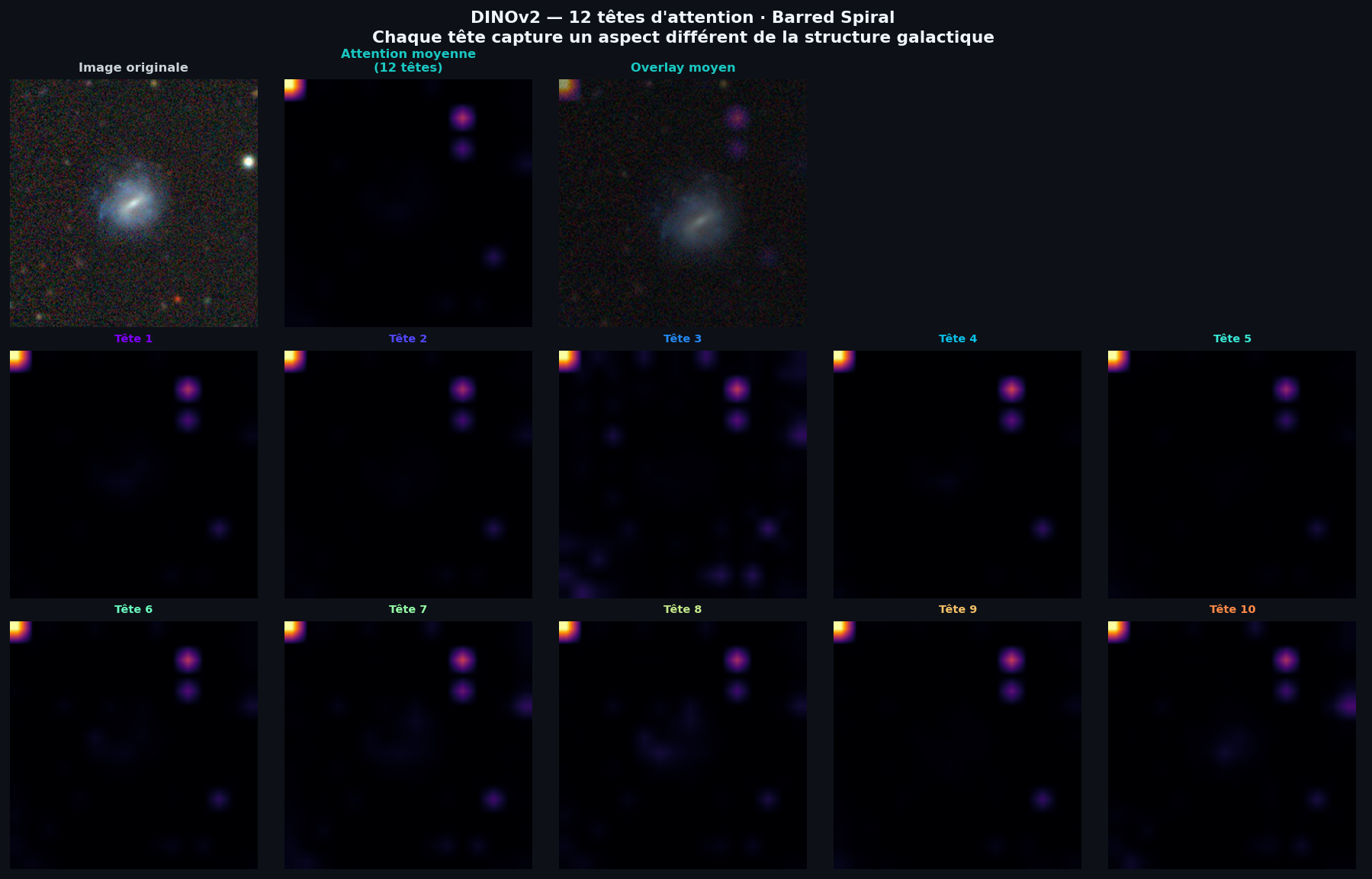
For the ViT the explanation is the CLS-token attention of the last block, averaged over the 12 heads and reshaped to the 16×16 patch grid (Caron et al. 2021). The qualitative observation of the project: with the frozen backbone, several heads attend to bright background stars; after fine-tuning, the attention covers the galaxy body. This is read from the figures, not quantified.
Attention-guided morphometry
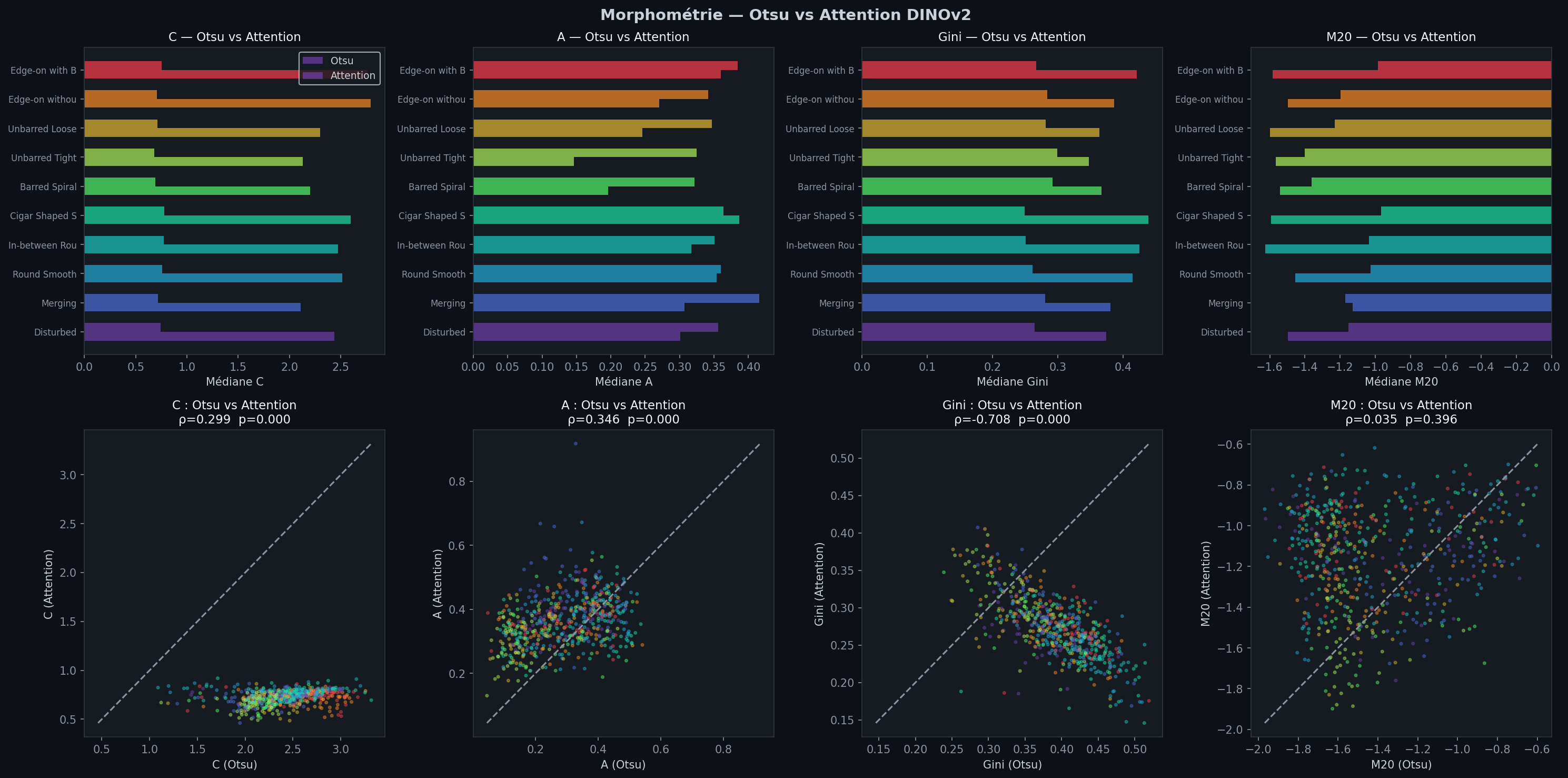
AttentionMorphometry replaces the Otsu mask of CAS/Gini/M20 with a mask from the fine-tuned DINOv2 attention map (threshold at the 60th percentile, holes filled) and recomputes the statistics on it. The aim is to define the galaxy region by structure rather than brightness. It was applied to 2,000 galaxies, 200 per class.
Do the statistics separate classes better?
A Kruskal–Wallis statistic across the ten classes measures class separation (larger = better):
| Statistic | Otsu mask | Attention mask |
|---|---|---|
| C (concentration) | 202.0 | 444.4 |
| A (asymmetry) | 100.9 | 229.3 |
| S (smoothness) | 150.8 | 305.9 |
| Gini | 177.8 | 311.2 |
| M20 | 61.6 | 373.0 |
_facts/astrovision/FACTS_INDEX.md §3 and shown when hovering over a number.The attention-based statistics have larger KW values for all five measures, most strikingly M20 (61.6 → 373.0).
The Otsu sample has 599 galaxies, the attention sample 2,000; a Kruskal–Wallis H grows with sample size, so part of the gap is a sample-size effect. The two C statistics also use different formulas. The result is suggestive of better class separation, not a measured improvement.
Medians by class (attention masks)
| Class | C | A | Gini | M20 | Components |
|---|---|---|---|---|---|
| 0 · Disturbed | 0.74 | 0.36 | 0.26 | −1.15 | 1 |
| 1 · Merging | 0.72 | 0.42 | 0.28 | −1.17 | 1 |
| 2 · Round Smooth | 0.76 | 0.36 | 0.26 | −1.03 | 1 |
| 3 · In-between Round Smooth | 0.77 | 0.35 | 0.25 | −1.04 | 1 |
| 4 · Cigar Shaped Smooth | 0.78 | 0.36 | 0.25 | −0.97 | 1 |
| 5 · Barred Spiral | 0.69 | 0.32 | 0.29 | −1.36 | 1 |
| 6 · Unbarred Tight Spiral | 0.68 | 0.33 | 0.30 | −1.40 | 1 |
| 7 · Unbarred Loose Spiral | 0.71 | 0.35 | 0.28 | −1.23 | 1 |
| 8 · Edge-on without Bulge | 0.71 | 0.34 | 0.28 | −1.20 | 1 |
| 9 · Edge-on with Bulge | 0.75 | 0.38 | 0.27 | −0.99 | 1 |
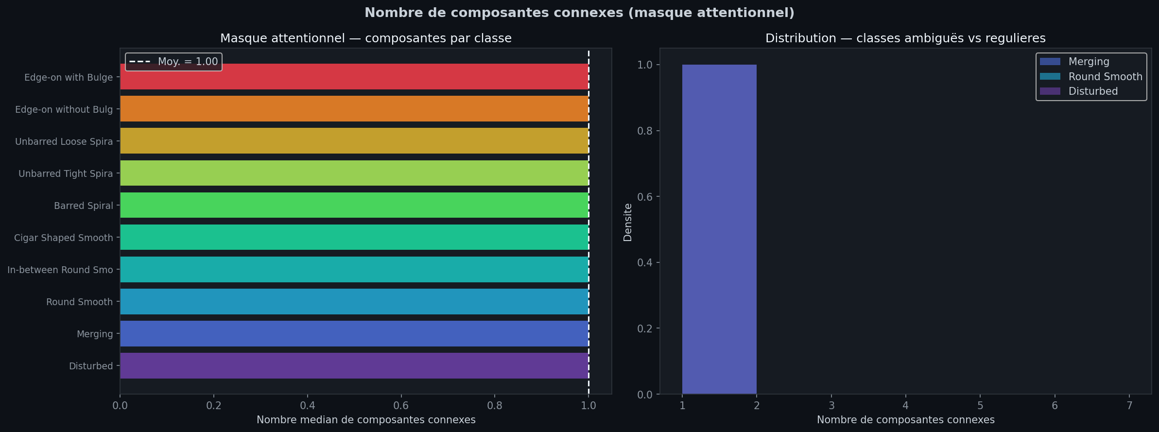
The median number of connected components is 1 even for Merging galaxies: a 16×16 attention map thresholded at a percentile yields one blob almost always, so the method cannot count multiple nuclei.
Link with colour
Correlations of the attention statistics with SDSS g−r are tiny: ρ = +0.070 for C and +0.087 for M20 (1,957 galaxies). Significant at p < 0.05 with this many galaxies, but explaining under 1 % of the variance.