Catalogue of 183 Spectral Features

This document catalogues the 183 spectroscopic features that form the central data matrix of the AstroSpectro project. They were extracted from N = 43,019 LAMOST DR5 spectra and validated by cross-matching with Gaia DR3. PCA, UMAP, t-SNE and the XGBoost classifier are all applied to this feature set.

PHY-3500 Context

This catalogue corresponds exactly to the dataset described in the Baker, Caillat & Jean report, "Does dimensionality reduction preserve the essential physical information of stellar spectra?", PHY-3500, Université Laval, 28 April 2026.


Overview​

Two reading levels​

The 183 features can be read according to two complementary frameworks.

The physical framework (6 families, used in the PHY-3500 report) groups features by the astrophysical observable they measure — this is the framework used to interpret PCA loadings and HDBSCAN clusters.

The technical framework (9 families, from the feature_engineering.py V2 module) reflects the code architecture — this is the framework useful for understanding how features are computed.

Distribution of the 183 features by physical family​

35
Balmer lines
Hα–Hθ
Teff — thermal axis PC1
PC1 29.7%
20
Ionised calcium
Ca II H&K + IR triplet
Metallicity + chromosphere
PC1 9.3%
15
Magnesium & α
Mg b, Mg 5184, [α/Fe]
[Mg/Fe], population I/II
30
Iron & metals
Fe, Cr, V, Ni, Ba, Sr...
[Fe/H] — metallicity axis PC2
PC2 79.7%
18
Lick/SDSS indices
Lick IDS, CaH, TiO
Age + composite metallicity
65
Continuum
Slopes, curvatures, colours
Teff (slope) · luminosity (breaks)
Each cell = 1 spectroscopic feature · 183 total · hover a family to highlight it
Exact count

The exact number of active features is determined at the first call to FeatureEngineer.extract_features() via _populate_feature_names() (stable alphabetical order). The feature_engineering.py V2 module declares 174 pure spectral features; the remaining 9 come from post-merge functions (add_gaia_derived_features, add_photometric_composites) called after cross-matching with the catalogue.


Spectral coverage — line positions on the LAMOST spectrum​

The visualisation below shows where each family's lines are located within the LAMOST spectral coverage (3,690–9,100 Å). The vertical bar indicates the separation between the blue and red arms of the spectrograph.

LAMOST DR5 spectral coverage — 3,690–9,100 Å — line-family positions
blue arm | red arm
H10
H9
H8
Hε
Hδ
Hγ
Hβ
Hα
Ca K
Ca H
IR1
IR2
IR3
Mg b
Fe
Fe
Fe
Na D
TiO
TiO
TiO
TiO
3690
4000
4500
5000
5500
6000
6500
7000
7500
8000
8500
9100
Balmer (H)
Ca II H&K + IR
Mg b
Iron & metals
Molecular bands
Å

Variables excluded from the PHY-3500 dataset​

Before any analysis, the following variables were removed from the initial dataset:

ra⦵
Angular coordinate
Geographic and instrumental observational bias.
dec⦶
Angular coordinate
Geographic and instrumental bias (redundant with RA).
redshift⤆
LAMOST metadata
Observational bias unrelated to intrinsic physical properties of the star.
spectro_only=True mode

In the supervised AstroSpectro pipeline, these variables are excluded via the spectro_only=True parameter of SpectralClassifier. They constitute an example of feature leakage: their discriminative power comes from the observation context, not from the intrinsic physical properties of the star. The published results (87% balanced accuracy, ROC-AUC ~0.964) use exclusively spectral features.


Detailed physical families​

Family 1 — Balmer lines (Hα–Hθ)​

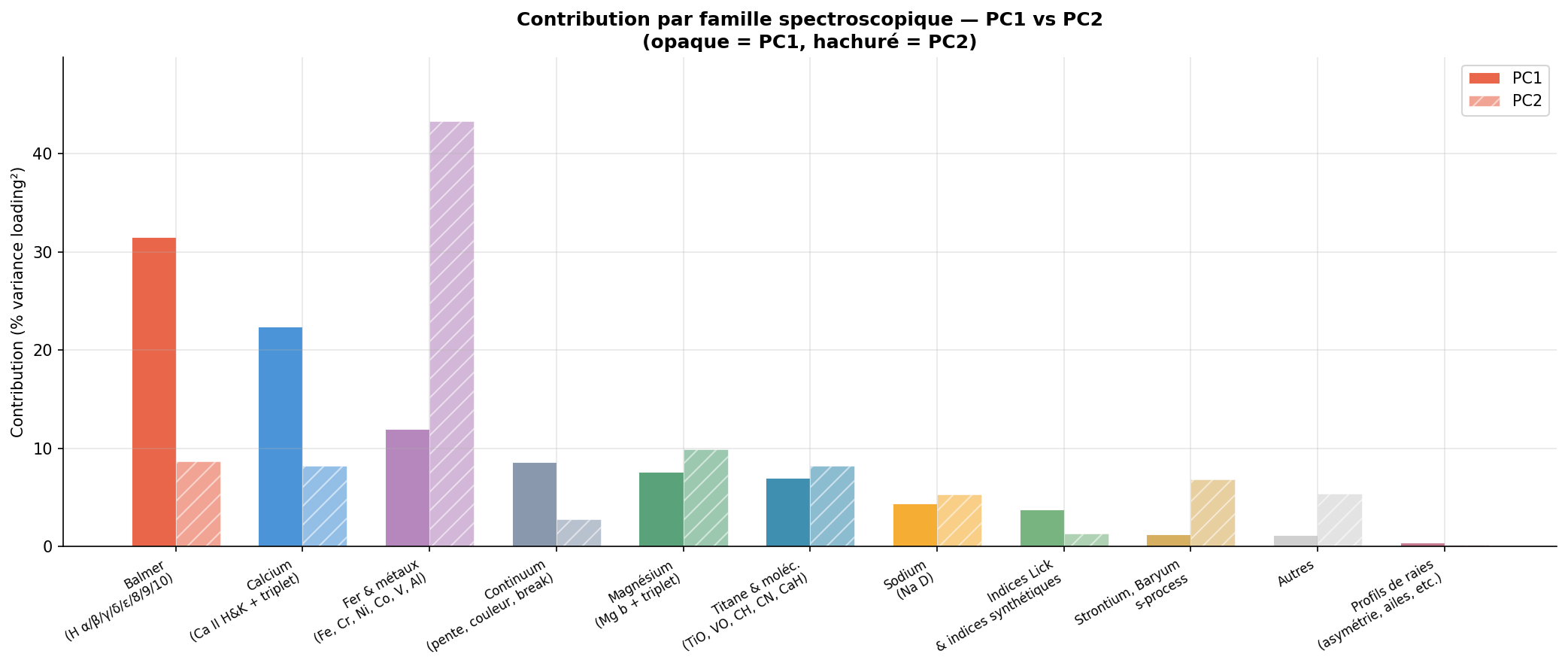
The Balmer series lines (transitions to the n=2 level of hydrogen) are the most powerful temperature indicators in the LAMOST spectral space. They contribute 31.5% of the variance of PC1 (thermal axis) in the PCA analysis of the 183-feature set.

Line
λ (Å)
Position
Extracted features
Hα
6562.8
prominence, FWHM, W(Hα), presence, full profile (10 metrics)
Hβ
4861.3
prominence, FWHM, W(Hβ), presence
Hγ
4340.5
W(Hγ), γ/β ratio
Hδ
4101.7
W(Hδ), δ/γ ratio
Hε
3970.1
prominence
H8
3889.0
prominence
H9
3835.4
prominence
H10
3797.9
prominence
Position in LAMOST spectrum 3690–9100 Å — Hα in the red, H10 in the near-UV

Extracted Balmer line ratios:

  • feature_balmer_ratio_gamma_beta: W(Hγ) / W(Hβ)
  • feature_balmer_ratio_delta_gamma: W(Hδ) / W(Hγ)
  • feature_balmer_temperature_index: (γ/β + δ/γ) / 2 — hot stars tend toward 1, cool stars exceed 1

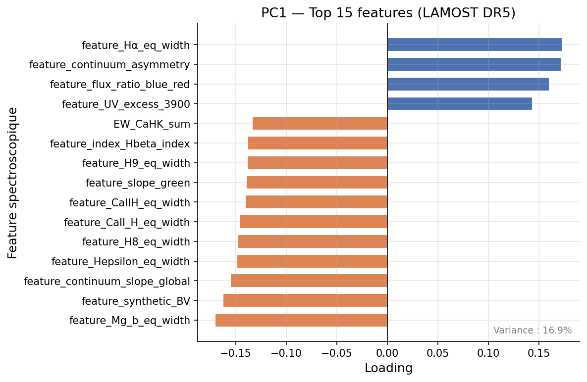
Link to PCA: ρ(PC1, Teff) = +0.831 (Spearman, N = 43,019). W(Hα) is the top absolute loading of PC1 (w = +0.173).


Family 2 — Ionised calcium — Ca II H&K and IR triplet​

The Ca II H (3968 Å) and K (3934 Å) lines are metallicity and surface gravity indicators. The IR triplet (8498, 8542, 8662 Å) is sensitive to the chromosphere and magnetic activity.

Line
λ (Å)
Species
Position
Extracted features
Ca II K
3933.7
Ca II
prominence, FWHM, W(CaIIK), full profile (10 metrics)
Ca II H
3968.5
Ca II
prominence, FWHM, W(CaIIH)
Ca 8498
8498.0
Ca II
EW via CaII_triplet index
Ca 8542
8542.1
Ca II
EW via CaII_triplet index
Ca 8662
8662.1
Ca II
EW via CaII_triplet index
H and K lines in the near-UV (LAMOST blue arm) · IR triplet in the deep red (red arm)

Composite Ca II indices:

  • EW_CaHK_sum: W(Ca II K) + W(Ca II H) — global metallicity proxy
  • ratio_EW_CaK_CaH: H/K equivalent width ratio
  • feature_ratio_prom_CaK_Hbeta: prominence(Ca II K) / prominence(Hβ) — robust temperature proxy

Contribution to PCA axes: Calcium contributes 22.4% of the variance of PC1 (second group after Balmer), confirming its role as a thermal indicator. The correlation ρ(PC1, [Fe/H]) = −0.548 shows that PC1 also captures part of the metallicity.


Family 3 — Magnesium and α-elements — Mg b, Mg 5184, [α/Fe]​

The Mg b triplet (around 5175 Å) and α-indices are sensitive to metallicity and the relative abundance of α-elements compared to iron — an indicator of the star's chemical history (populations I/II).

Line / Index
λ (Å)
Position
Extracted features
Mg b
5175.0
prominence, FWHM, W(Mg b) — triplet 5167/5173/5184 Å
Mg b Lick
5175.0
Lick index feature_index_Mgb_index · window 5160–5190 Å
Mg 1 Lick
5102.0
feature_index_Mg_1 · window 5069–5135 Å
Mg 2 Lick
5176.0
feature_index_Mg_2 · window 5154–5197 Å
Mg b triplet at ~5175 Å — visible mid-range · [Mg/Fe] and stellar population indicator

Ratios involving Mg b:

  • feature_ratio_prom_Mgb_Hbeta: prominence(Mg b) / prominence(Hβ)
  • ratio_EW_MgB_NaD: ratio W(Mg b) / W(Na D)
  • contrast_metals_vs_balmer: Mg/Ca vs Balmer contrast — [Fe/H] proxy

Composite proxies:

  • feature_FeH_proxy: estimated from the combined metallicity index
  • feature_alpha_Fe_proxy: log10(α_index / iron_index), bounded between −0.5 and +0.5

Family 4 — Iron peak metals — Fe, Cr, V, Ni, Ba, Sr, Al, Co​

This family groups iron-peak element lines, sensitive to overall metallicity [Fe/H]. It dominates PC2 with 43.3% of the variance — PC2 is the metallicity axis of the feature set.

Strength:
strong
medium
weak
· Bar shows λ position in 3690–9100 Å
Fe
Iron · Fe I / Fe II
6 lines
4383.5 Å
Fe I
4531.1 Å
Fe II
5270.4 Å
Fe I
5335.2 Å
Fe I
5406.8 Å
Fe I
5709.4 Å
Fe I
→ PC2 loading +0.174
Cr
Chromium · Cr I
2 lines
5206.0 Å
Cr I
5208.4 Å
Cr I
Ni
Nickel · Ni I
1 line
5081.1 Å
Ni I
Na
Sodium · Na I
2 lines
5889.9 Å
Na I
5895.9 Å
Na I
→ D doublet — ratio W(MgB)/W(NaD)
Ba
Barium · Ba II
2 lines
4554.0 Å
Ba II
6496.9 Å
Ba II
Sr
Strontium · Sr II
1 line
4077.7 Å
Sr II
Si
Silicon · Si II
2 lines
4128.1 Å
Si II
4130.9 Å
Si II
Ti
Titanium · Ti II
2 lines
4758.1 Å
Ti II
4764.9 Å
Ti II
→ α-elements proxy
Al
Aluminium · Al I
1 line
3944.0 Å
Al I
Co
Cobalt · Co I
1 line
5301.0 Å
Co I
V
Vanadium · V II
1 line
4379.2 Å
V II
For each line: prominence, FWHM and W(line) via specutils.analysis.equivalent_width. Composites: feature_metal_index_combined, feature_iron_peak_index, feature_alpha_elements_index.

Family 5 — Composite metallicity indices — Lick, SDSS, CaII triplet​

Spectral indices are standardised flux measurements in narrow spectral windows, computed relative to a local pseudo-continuum. They allow direct comparisons with stellar population libraries (Lick/IDS, SDSS).

Filter by origin:
position in 3690–9100 Å
Index
λ window
Origin
Observable
TiO 5
7126–7135 Å
Lick
TiO bands — cool M stars
Dn4000
4000–4100 Å
standard
4000 Å break — age / metallicity
Dn4000 SDSS
4050–4250 Å
SDSS
Extended version of the D4000 break
G4300
4280–4320 Å
Lick
CH band — G subgiants
Ca4227
4225–4235 Å
Lick
Ca I — metallicity
Hβ index
4840–4870 Å
Lick
Hβ — stellar age
Mgb index
5160–5190 Å
Lick
Mg b — [Mg/Fe]
Ca II triplet
8480–8680 Å
standard
Ca II IR — gravity / activity
CaH 2
6814–6846 Å
standard
CaH — M subtypes
CaH 3
6960–6990 Å
standard
CaH — M subtypes
CN 1
4142–4177 Å
Lick
CN — giants / stellar evolution
CN 2
4216–4251 Å
Lick
CN — giants / stellar evolution
Mg 1
5069–5135 Å
Lick
[Mg/Fe]
Mg 2
5154–5197 Å
Lick
[Mg/Fe]
Na D Lick
5876–5909 Å
Lick
Na D — gravity / age
TiO 1 Lick
5936–5994 Å
Lick
TiO — cool stars
TiO 2 Lick
6190–6272 Å
Lick
TiO — cool stars
Paschen 12
8730–8772 Å
standard
Paschen series

Family 6 — Continuum features — slopes, curvatures, jumps, colours​

Continuum features capture the global spectral morphology without focusing on individual lines. They encode effective temperature (slope and colour), luminosity class (jumps), and observation quality.

Local slopes (sigma-clipped, σ = 2.5)​

〜Local slopes — sigma-clipped (σ = 2.5)5 features
Feature
Position 3690–9100 Å
Interpretation
feature_slope_blue
UV — hot stars
negative = blue spectrum
feature_slope_green
Mid visible
feature_slope_red
Red visible
feature_slope_deep_red
Near-IR — cool stars
feature_continuum_slope_global
Global blue/red slope
∪Local curvatures — Savitzky-Golay (second derivative)3 features
Feature
Centre
Interpretation
feature_curvature_4000
4000 Å
4000 Å break — age/metallicity boundary
feature_curvature_5000
5000 Å
Mid visible — blackbody curvature
feature_curvature_6000
6000 Å
Red — transition to IR
↑Spectral breaks — continuum discontinuities5 features
Feature
Description
Status
feature_paschen_jump_strength
Paschen jump 8120/8220 Å
Luminosity class
✓ active
feature_break_4000A_strength
D4000 break strength
Age / metallicity
✓ active
feature_break_4000A_width
D4000 break width
Age / metallicity
✓ active
feature_balmer_jump_strength
Balmer jump 3646 Å
NaN — outside LAMOST coverage
✗ NaN
feature_brackett_jump_strength
Brackett jump 14,500 Å
NaN — outside LAMOST coverage
✗ NaN
≈Asymmetry and synthetic colours7 features
Feature
Formula
Interpretation
feature_continuum_asymmetry
(f_blue − f_red) / (f_blue + f_red)
Blue/red asymmetry
feature_flux_ratio_blue_red
f_blue / f_red
B/R flux ratio
feature_UV_excess_3900
f(3850–3950) / f(4400–4600)
UV excess — A stars
feature_color_index_BlueRed
derived from flux
Global colour proxy
feature_color_gr
magnitude g − r
LAMOST g−r colour
feature_color_ri
magnitude r − i
LAMOST r−i colour
feature_synthetic_BV
computed from spectrum
Synthetic B−V proxy
All continuum features are computed on the normalised spectrum after sigma-clipping. NaN values correspond to wavelengths outside LAMOST coverage (3,690–9,100 Å).

Molecular bands — TiO, VO, CN, CH, CaH, MgH​

Molecular bands are the spectral signatures of the coolest stars (late K and M types). They appear in the HDBSCAN clusters corresponding to K-M dwarfs in UMAP space.

Band positions in 3690–9100 Å
4000
5000
6000
7000
8000
9000
TiO
Titanium oxide
K–M
M stars — late K dwarfs
TiO 6180
6155–6255 Å
TiO 7050
7000–7200 Å
TiO 7600
7550–7750 Å
TiO 8200
8150–8350 Å
TiO 8400
8350–8550 Å
TiO 8860
8835–8935 Å
VO
Vanadium oxide
M
Coolest M stars
VO 7400
7325–7625 Å
VO 7900
7825–8125 Å
CN
Cyanide
Giants
Giants — stellar evolution
CN 4142
4125–4195 Å
CN 8200
8150–8350 Å
CH
Methylidyne
G
G band — G subgiants
CH 4300
4280–4330 Å
CaH
Calcium hydride
M
M subtypes — cool dwarfs
CaH 6380
6375–6395 Å
CaH 6830
6825–6845 Å
CaH 6975
6970–6990 Å
MgH
Magnesium hydride
K–M
Cool stars / metallicity
MgH 5140
5135–5155 Å
Feature extracted per band: ratio flux_band / flux_continuum. These bands appear in the HDBSCAN clusters corresponding to K-M dwarfs in UMAP space.

Correlations with Gaia DR3 parameters​

The following table presents Spearman correlations between PC1/PC2 and Gaia DR3 astrophysical parameters (N = 43,019 stars). Colour intensity reflects |ρ| — hover over a cell to see the interpretation.

Colour intensity ∝ |ρ| :
strong positive
strong negative
moderate
weak
Gaia DR3 Parameter
Unit
ρ(PC1, ·)
ρ(PC2, ·)
Teff
K
+0.831
+0.156
log g
dex
-0.155
+0.081
[Fe/H]
dex
-0.548
-0.082
G_BP − G_RP
mag
-0.768
-0.025
SNR_r
+0.071
-0.310
A_G
mag
-0.070
+0.196
PC1 = thermal axis — ρ(Teff) = +0.831. Continuous Teff gradient (hot A-F stars on the right, cool K-M on the left).
PC2 = metallicity axis — metal indices lead its loadings. ⚠️ Partially contaminated by SNR (ρ = −0.310): instrumental artefact inherent to unsupervised PCA.

Top-5 loadings of PC1 and PC2​

Extracted from the PHY-3500 report, Table 2. Signed bars show the direction and amplitude of each feature's contribution to its principal axis.

PC1
thermal axis · 16.9% variance · ρ(Teff) = +0.831
interpretation
Temperature T_eff
#
Feature
← negative · · · · positive →
w
1
Hα EW
+0.173
2
continuum asymmetry
+0.172
3
Mg b EW
-0.171
4
synthetic BV
-0.163
5
flux ratio blue red
+0.161
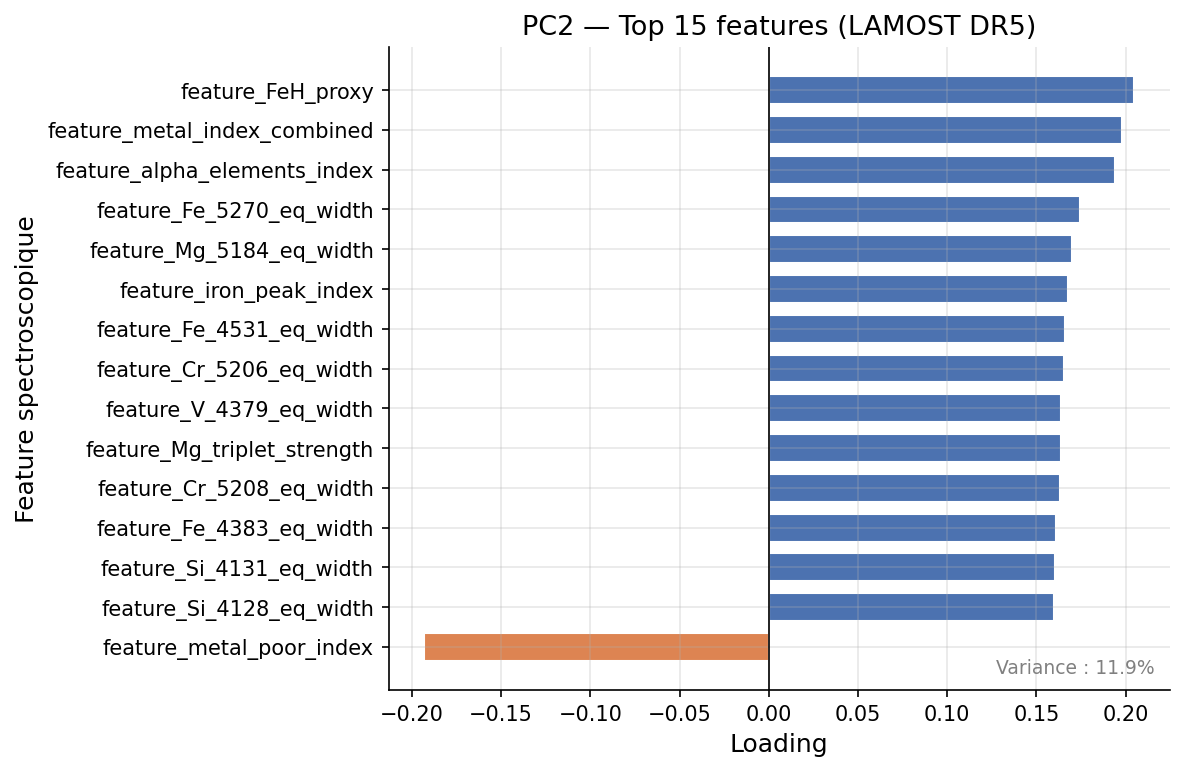
PC2
metallicity axis · 11.9% variance
interpretation
Metallicity [Fe/H]
#
Feature
← negative · · · · positive →
w
1
FeH proxy
+0.205
2
metal index combined
+0.198
3
alpha elements index
+0.194
4
metal poor index
-0.193
5
Fe 5270 EW
+0.174

Reference figures​

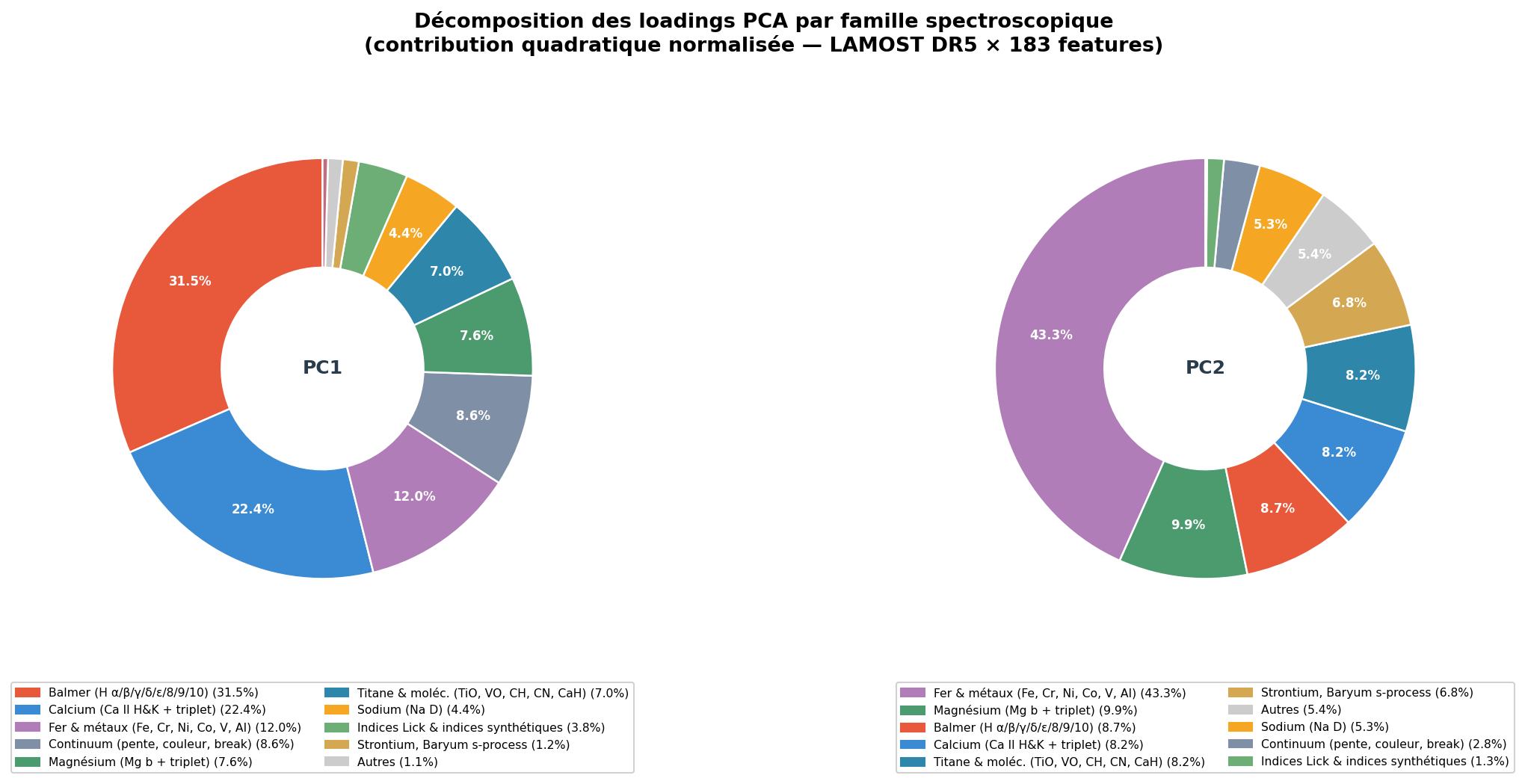
The following figures illustrate the relative importance of feature families and the PCA loading structure. Click an image to enlarge.
◎
Family contributions — PC1 vs PC2
PCA loadings
Family contributions — PC1 vs PC2
Normalised quadratic contribution — Balmer dominates PC1, Fe/metals dominate PC2
◎
Donut distribution by family
PCA loadings
Donut distribution by family
Circular view of relative contributions PC1 (left) and PC2 (right)
◎
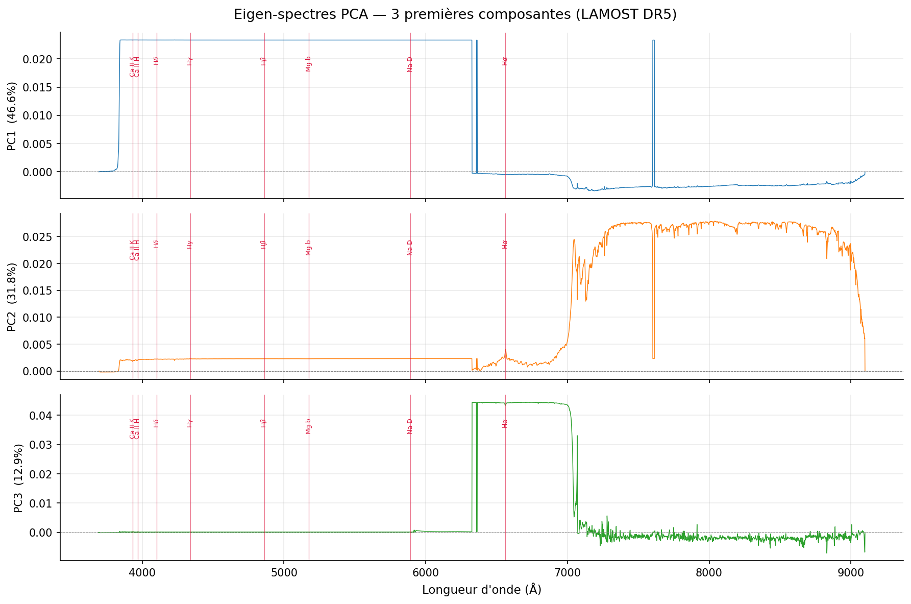
PCA eigenspectra on raw flux
Raw flux
PCA eigenspectra on raw flux
PC1 = Teff slope · PC2 = IR rise cool stars · PC3 = instrumental cut
◎
Top loadings PC1 — thermal axis
PC1 · Teff
Top loadings PC1 — thermal axis
W(Hα) at top (w = +0.173) · Balmer + Ca II + continuum dominate
◎
Top loadings PC2 — metallicity axis
PC2 · [Fe/H]
Top loadings PC2 — metallicity axis
[Fe/H]proxy at top (w = +0.205) · All chemical composition indicators
◎
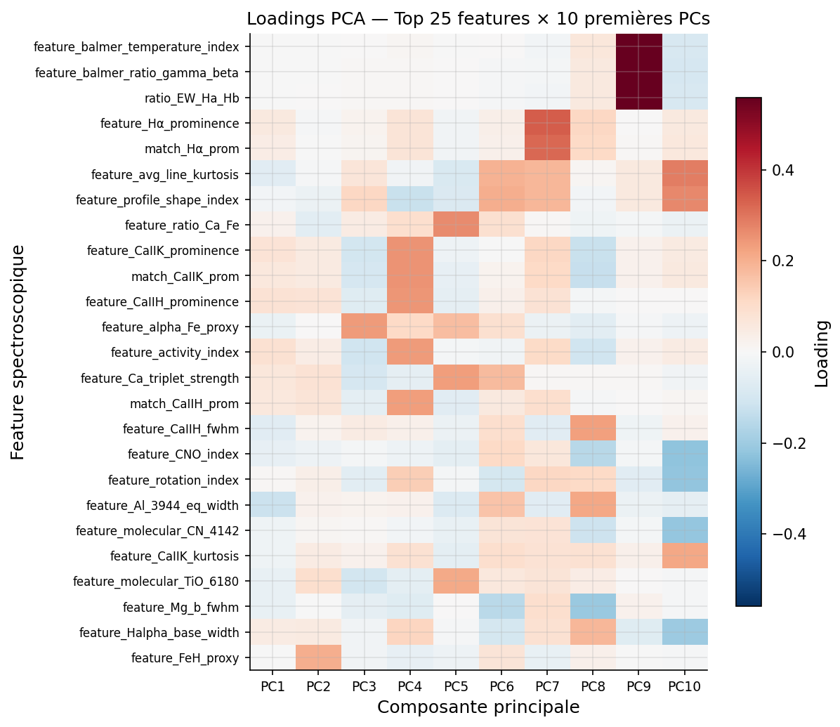
Complete loadings heatmap
Heatmap 183×K
Complete loadings heatmap
Matrix 183 features × K components — structure and eigenspectrum decay

Code reference​

from src.pipeline.feature_engineering import FeatureEngineer

fe = FeatureEngineer()

# Extraction for one spectrum
vec = fe.extract_features(matched_lines, wl, flux_norm, invvar)

# Number of features (determined at first call)
print(len(fe.feature_names)) # → 174 (pure spectral)

# Post-merge: add derived Gaia features
from src.pipeline.feature_engineering import (
add_gaia_derived_features,
add_photometric_composites,
add_line_composites,
)

df, new_cols = add_gaia_derived_features(df) # bp_g, M_G, v_tan, etc.
df, mod_cols = add_photometric_composites(df) # bp_g, color_ug, Q_parameter
df, lc_cols = add_line_composites(df) # EW_CaHK_sum, EW/FWHM ratios

To activate pure spectroscopic mode (without Gaia, without redshift/ra/dec):

from src.pipeline.classifier import SpectralClassifier

clf = SpectralClassifier(model_type="XGBoost", prediction_target="main_class")
clf.train_and_evaluate(features_df, spectro_only=True)