Autoencoder — Non-linear Dimensionality Reduction
This page documents the results of the SpectralAutoencoder neural autoencoder applied to the 183 spectroscopic features of N = 43,019 LAMOST DR5 × Gaia DR3 spectra. The autoencoder is the third dimensionality reduction method studied in the PHY-3500 project, complementing PCA (linear) and UMAP/t-SNE (non-parametric). Its role is to provide a non-linear parametric representation: it learns a compression and can project new spectra without full recomputation.
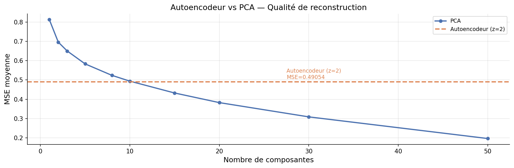
The autoencoder is mentioned in the Baker, Caillat & Jean article (28 April 2026) but its detailed results are not developed in the main text — the reader is referred to this documentation page. Key results: MSE(AE, z=2) = 0.489 ≈ PCA(k=10), and the discovery that latent axis 1 encodes gravity rather than temperature.
Key results
Why an autoencoder?
Previous methods have complementary limitations:
| Method | Linear? | Parametric? | Main advantage | Limitation |
|---|---|---|---|---|
| PCA | ✓ | ✓ | Interpretable loadings · reproducible | Blind to non-linear relationships |
| UMAP / t-SNE | ✗ | Partial | Topological structure · clusters | No exact transform() for new points |
| Autoencoder | ✗ | ✓ | Non-linear + parametric | Black box · training cost |
The autoencoder is non-linear (it can capture structures that PCA flattens) and parametric (once trained, encoding a new spectrum is a simple forward pass). This is the ideal combination for a production pipeline.
Architecture
Justification of architecture choices
Symmetric MLP (183 → 256 → 128 → 64 → 2 → 64 → 128 → 256 → 183): The initial expansion to 256 (> 183) is not an error — it allows the network to create richer intermediate representations before compression. This is common practice for autoencoders on spectral data (Portillo et al. 2020, AJ 160:45).
BatchNorm + Dropout(p=0.1): BatchNorm stabilises gradients and accelerates convergence. Light dropout (0.1) avoids overfitting without degrading reconstruction — stellar spectra are regular enough that stronger dropout is counterproductive.
Latent dimension z = 2: Deliberate choice for 2D visualisation and fair comparison with PCA(k=2) and UMAP(2D). A z = 8 or 16 would achieve much lower MSE but would lose visual readability.
from src.dimred.autoencoder import SpectralAutoencoder

# Training
ae = SpectralAutoencoder(input_dim=183, latent_dim=2, hidden_dims=[256, 128, 64])
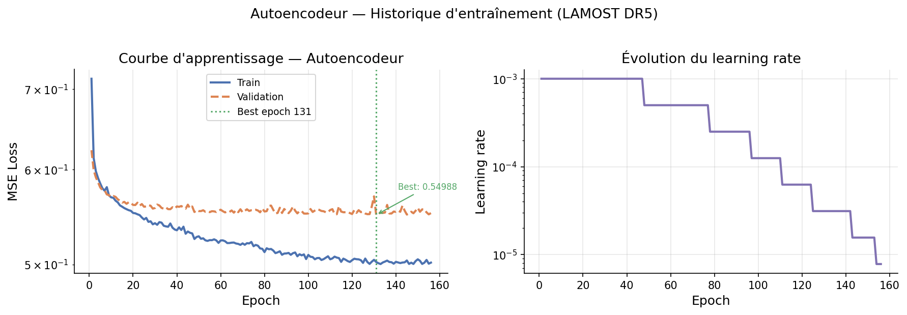
history = ae.fit(X_train_scaled, epochs=200, lr=1e-3, batch_size=512, patience=15)

# Encode 43,019 spectra → 2D latent space
Z_ae = ae.encode(X_scaled)   # shape: (43019, 2)

# Reconstruction
X_recon = ae.decode(Z_ae)    # shape: (43019, 183)
mse = ae.reconstruction_mse(X_scaled)  # → 0.489
Reconstruction — Autoencoder vs PCA
MSE(k) benchmark
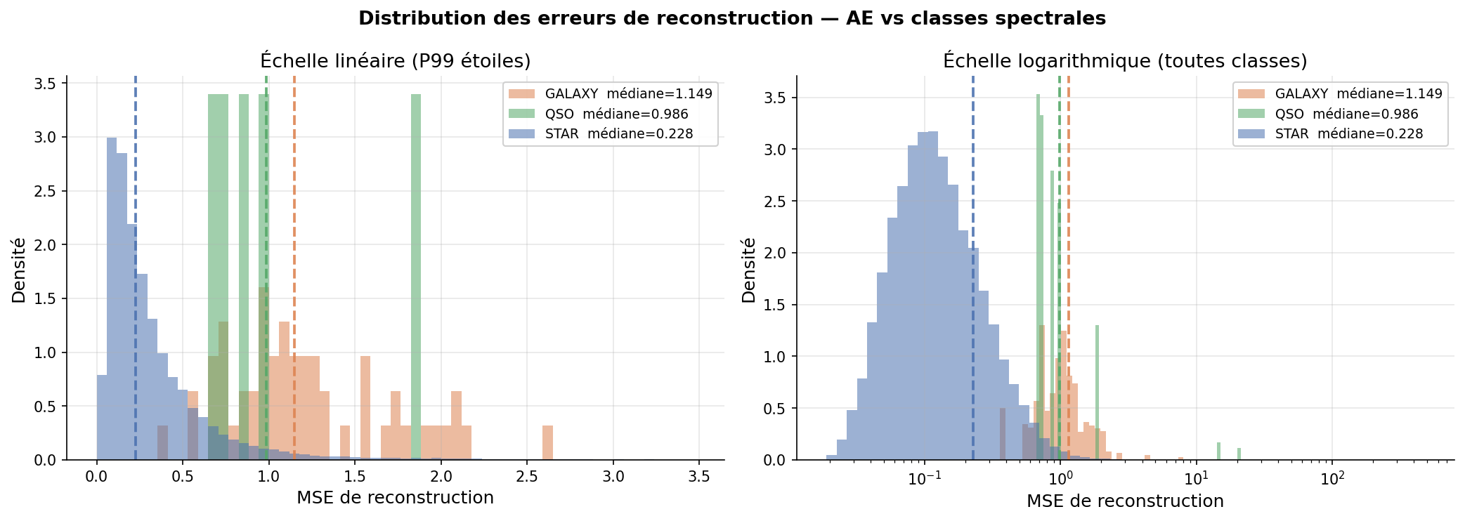
Reconstruction error by object type
The per-class breakdown reveals an important astrophysical result:
| Class | N | Mean MSE | Median MSE | p95 | Factor vs stars |
|---|---|---|---|---|---|
| STAR | 42,956 | 0.485 | 0.227 | 0.974 | 1× (reference) |
| GALAXY | 56 | 3.009 | 1.170 | 3.043 | ~5× |
| QSO | 7 | 5.794 | 0.954 | 18.637 | ≈ 4.2× (median) · ≈ 11.9× (mean) |
With only 7 QSOs in the sample, the ratios are fragile. QSOs (quasi-stellar objects) have a median reconstruction error about 4.2× that of stars (0.954 / 0.227) and a mean error about 11.9× (5.794 / 0.485). The autoencoder, trained almost exclusively on stars (99.85% of the sample), has never learned the spectral structure of QSOs — their broad emission lines (Ly-α, CIV) are radically different. This result suggests that reconstruction error can serve as an anomaly score: a spectrum with MSE >> 1 is likely non-stellar.
Latent space and physical interpretation
Spearman correlations with Gaia DR3
Latent space organisation
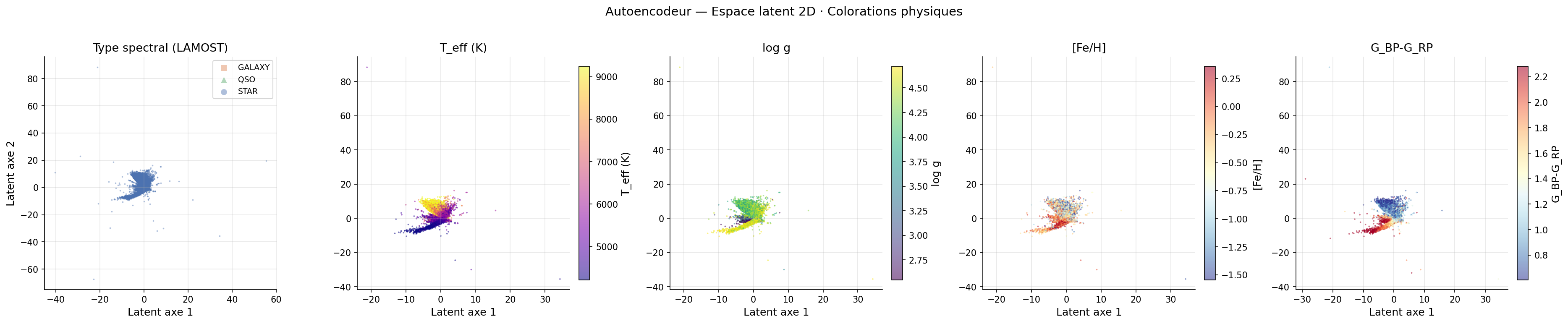
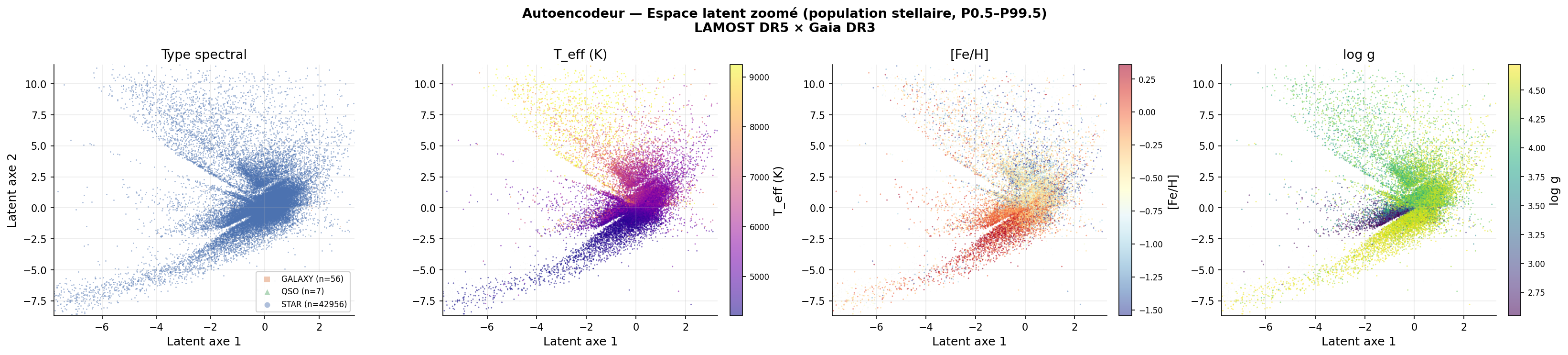
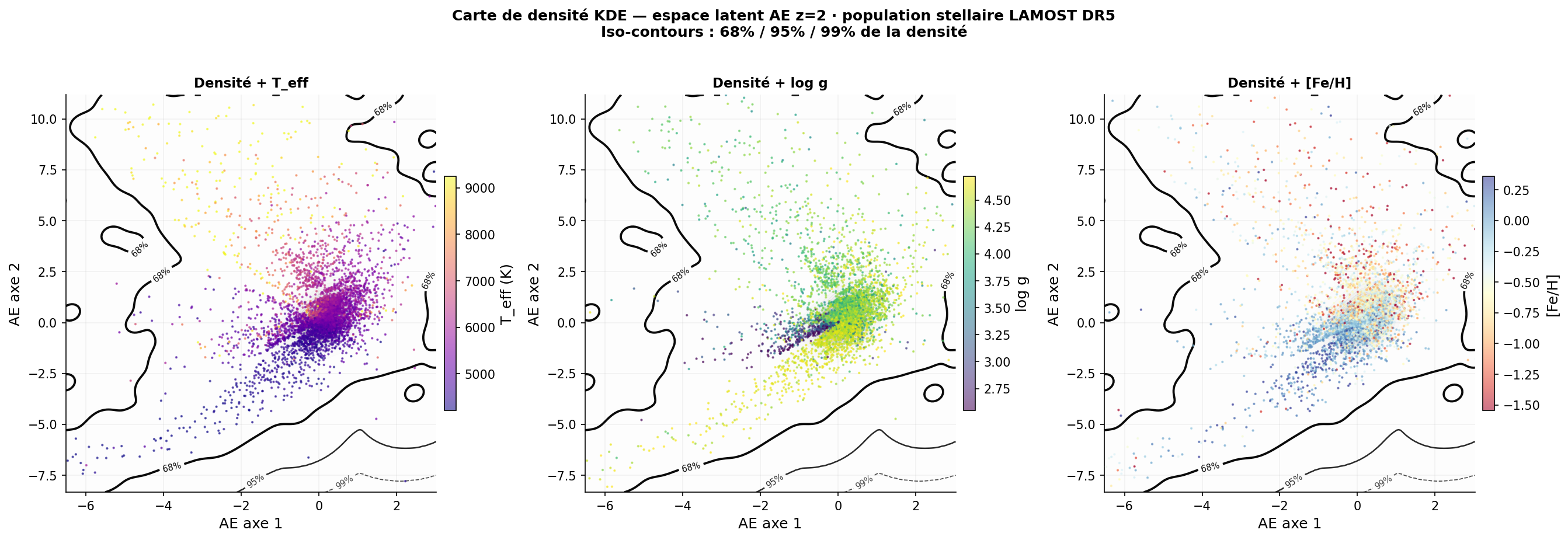
The latent space grid (ae_latent_grid.png) reveals a physically coherent organisation:
- Axis 2 (thermal, ρ = +0.793 with Teff) deploys the M-K-G-F-A sequence from bottom to top
- Axis 1 (gravity, ρ = +0.340 with log g) separates dwarfs and giants
- Galaxies and QSOs are pushed far from the main stellar mass — their high reconstruction error corresponds to their distance in latent space
This result is an independent confirmation of the HDBSCAN discovery: the dwarf/giant distinction is a genuine physical dimension of spectral space.
Latent space interpolation
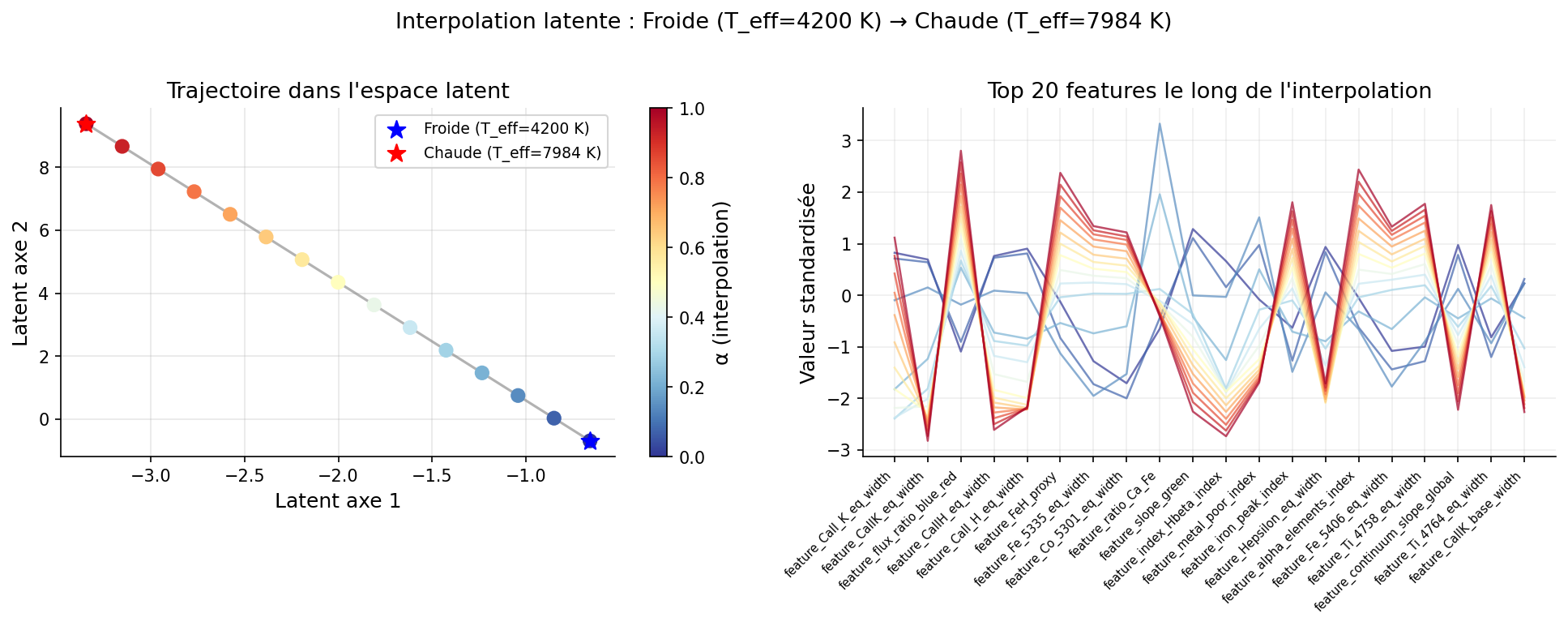
The parametric autoencoder allows linear interpolation between two points in latent space and decoding intermediate positions into physical spectra:
# Interpolation between a cool star (K) and a hot star (A)
# idx_cold: Teff = 4,200 K · idx_hot: Teff = 7,984 K
# Latent distance = 11.44 units

t = np.linspace(0, 1, 10)
Z_interp = np.outer(1-t, Z_ae[idx_cold]) + np.outer(t, Z_ae[idx_hot])
X_interp = ae.decode(Z_interp)
# → 10 synthetic intermediate spectra between 4,200 and 7,984 K
The interpolation produces a continuous and physically plausible transition: Balmer lines progressively weaken and Ca II lines strengthen. The latent distance of 11.44 units for a Teff variation of ~3,800 K confirms that axis 2 linearly encodes temperature.
Latent arithmetic — Stellar analogies
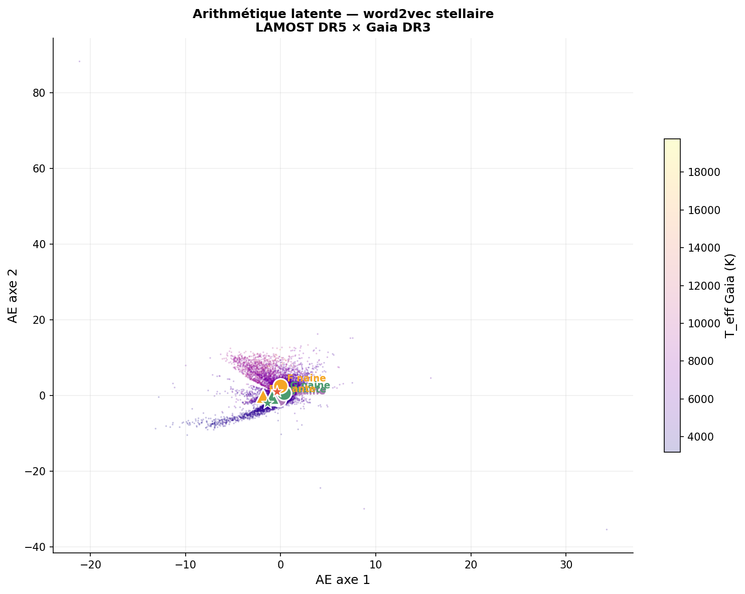
Following the word2vec idea (Mikolov et al. 2013), does the latent space support analogies of the type K_giant − K_dwarf + G_dwarf ≈ G_giant?
# K_giant − K_dwarf + G_dwarf = ?
z_pred  = z_K_giant - z_K_dwarf + z_G_dwarf
z_target = z_G_giant

distance = np.linalg.norm(z_pred - z_target)
# → distance = 2.1 (= ~18% of total range) — FUNCTIONAL ANALOGY
The result indicates that the latent space encodes the dwarf↔giant direction consistently across spectral types — suggesting the network has learned a representation that partially factorises (temperature, gravity) in a measurable way.
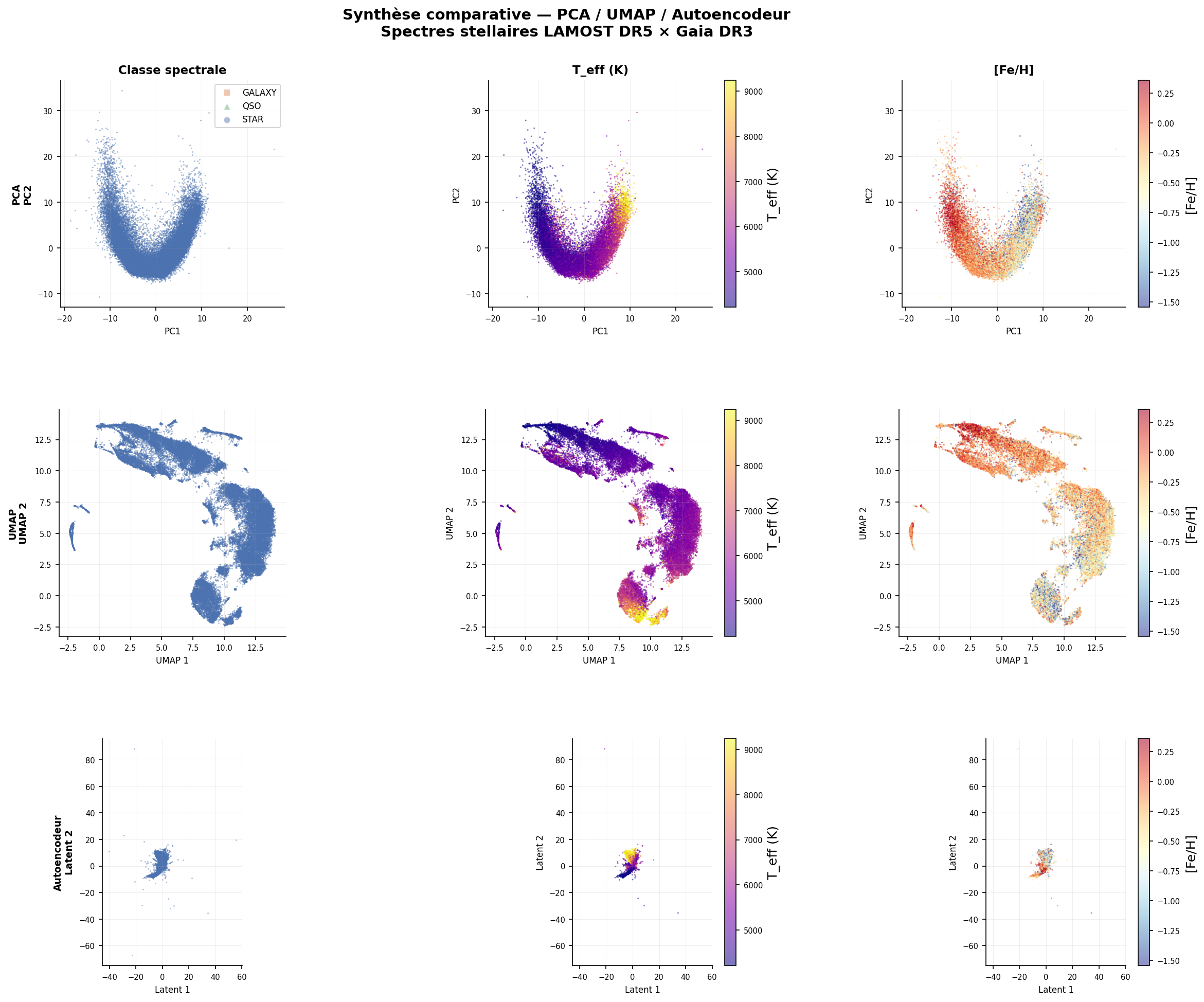
Comparative synthesis — PCA · UMAP · Autoencoder
| Criterion | PCA (z=2) | AE (z=2) | UMAP (2D) |
|---|---|---|---|
| Reconstruction MSE (2 dim) | 0.696 | 0.489 | N/A |
| Axis 1 / Teff correlation | +0.831 | +0.019 | +0.464 |
| Dominant physical axis | Temperature | Gravity | Temperature |
| Non-linear | ✗ | ✓ | ✓ |
| Parametric (transform) | ✓ | ✓ | Partial |
| Interpretable | ✓ (loadings) | ~ (correlations) | ✗ |
| Anomaly detection | ✓ (high MSE) | ✓ (QSO median MSE ≈ 4× stars, N = 7) | ✗ directly |
Reference figures
Diagnostic sheets — typical candidates
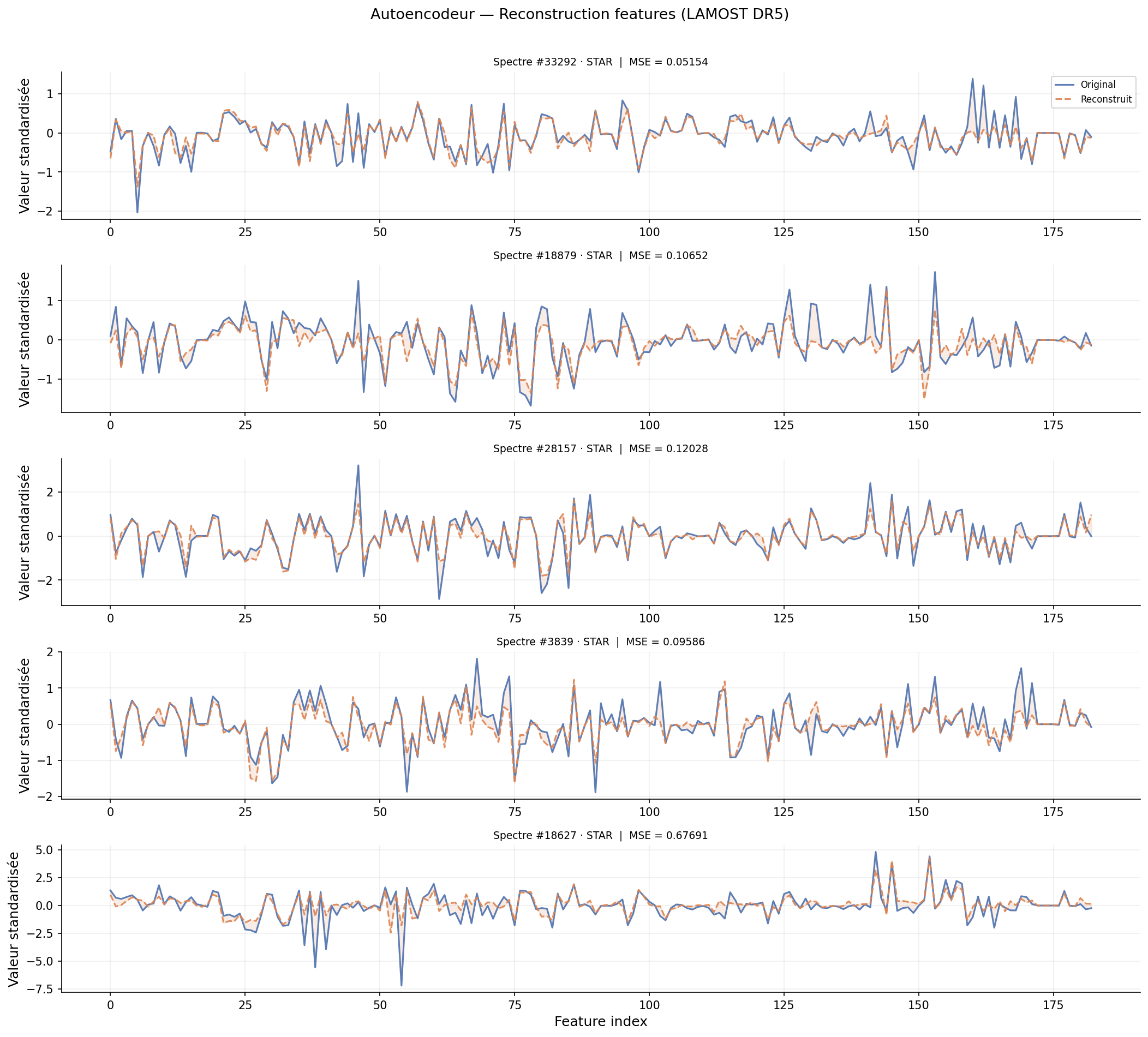
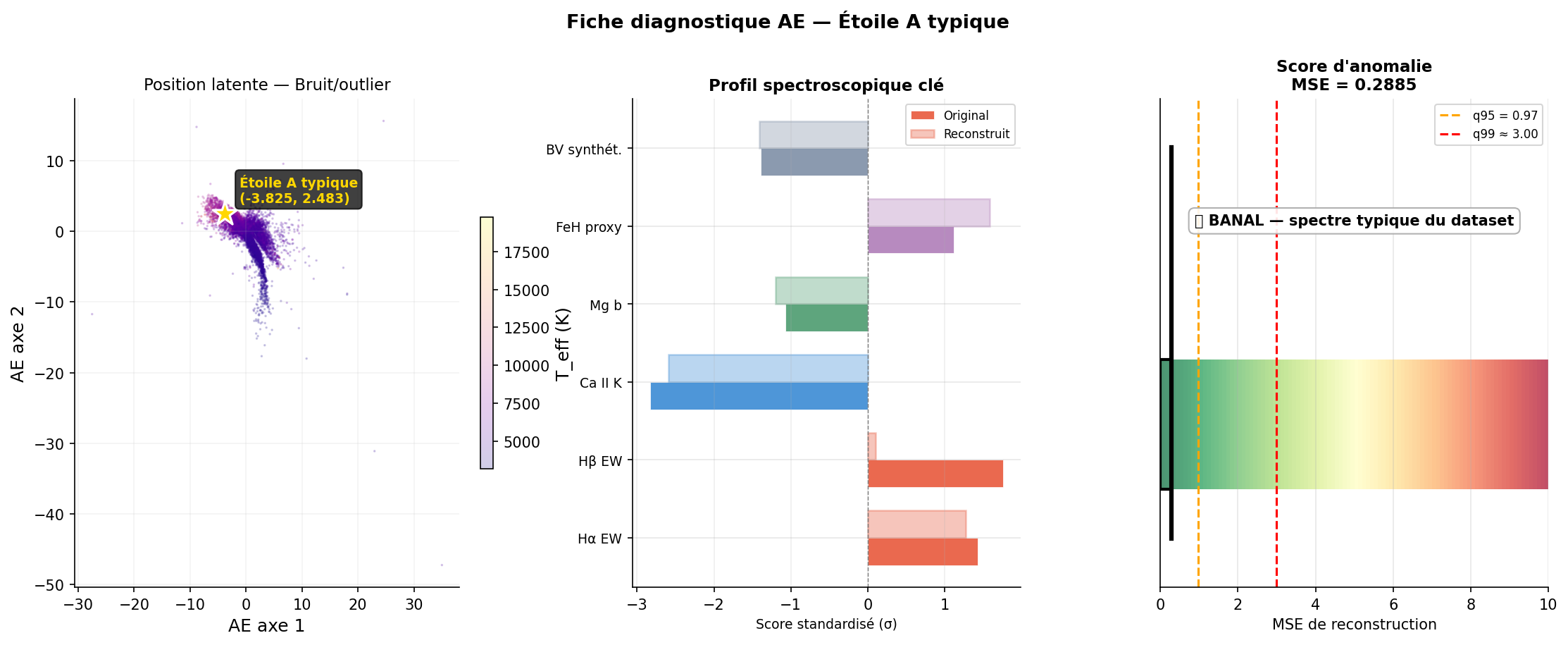
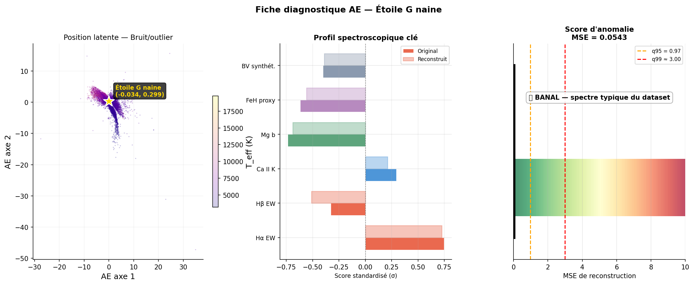
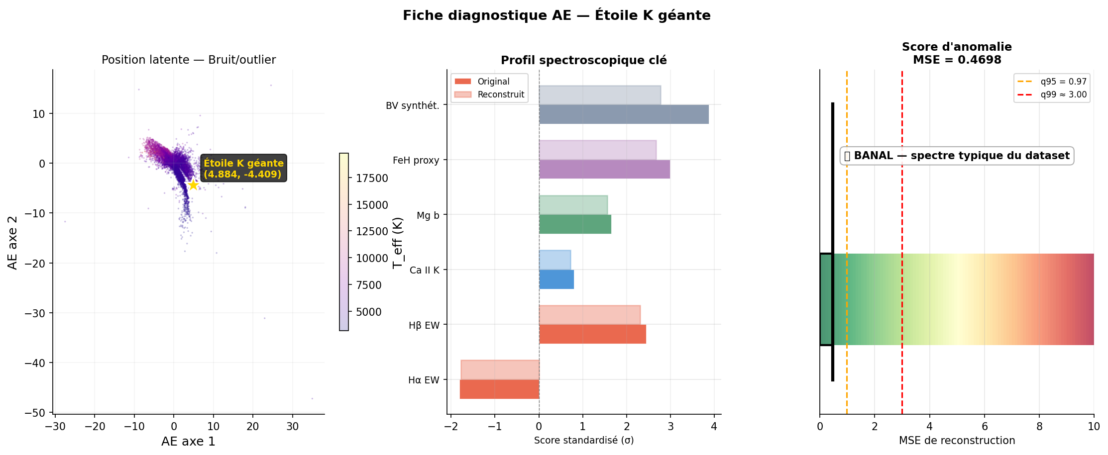
The autoencoder allows producing a diagnostic sheet for each spectrum: position in latent space, original vs reconstructed spectrum, residual, and MSE. Three characteristic examples:
Implementation
Code is in src/dimred/autoencoder.py (class SpectralAutoencoder) and the complete notebook in phy3500_03_autoencoder.ipynb.
# Load saved model
import torch
from src.dimred.autoencoder import SpectralAutoencoder

ae = SpectralAutoencoder(input_dim=183, latent_dim=2)
ae._model = torch.load("data/reports/models/ae_latent2.pt")
ae._model.eval()

# Encode a new spectrum
X_new_scaled = scaler.transform(X_new)  # same scaler as at training
Z_new = ae.encode(torch.tensor(X_new_scaled, dtype=torch.float32).numpy())