PCA vs UMAP vs t-SNE vs AE — Comparison
Dataset
PHY-3500 · G1 · 43,019 spectra — PCA run phy3500_pca_run_20260408T012751Z, UMAP / t-SNE run phy3500_umap_tsne_run_20260405T214233Z, autoencoder run phy3500_autoencoder_run_20260405T220839Z. Nothing on this page comes from the G2 runs.
Quantitative comparison
| Metric | PCA | UMAP | t-SNE | Autoencoder |
|---|---|---|---|---|
| Reconstruction MSE (K=2) | 0.696 | — | — | 0.489 |
| ρ(axis 1, T_eff) | +0.831 | +0.464 | — | +0.019 |
| Procrustes stability dP | 0 (exact) | 3.0 × 10⁻² | 5.0 × 10⁻⁴ | — |
| CPU time (Ryzen 9 5950X) | < 1 s | 40.1 s | 80.2 s | 143.7 s |
| Parametric | ✓ | Partial | ✗ | ✓ |
| Non-linear | ✗ | ✓ | ✓ | ✓ |
| Interpretable axes | ✓ | ✗ | ✗ | ✗ |
| Latent generation | Partial | ✗ | ✗ | ✓ |
When to use each method
| Method | Best for |
|---|---|
| PCA | Interpretable linear baseline; axis physical meaning; input to UMAP/t-SNE |
| UMAP | Topological structure; continuous gradients; HDBSCAN clustering |
| t-SNE | Sharp discrete cluster separation; stability; subpopulation isolation |
| Autoencoder | Non-linear compression; anomaly detection; latent arithmetic |
Synthesis figure
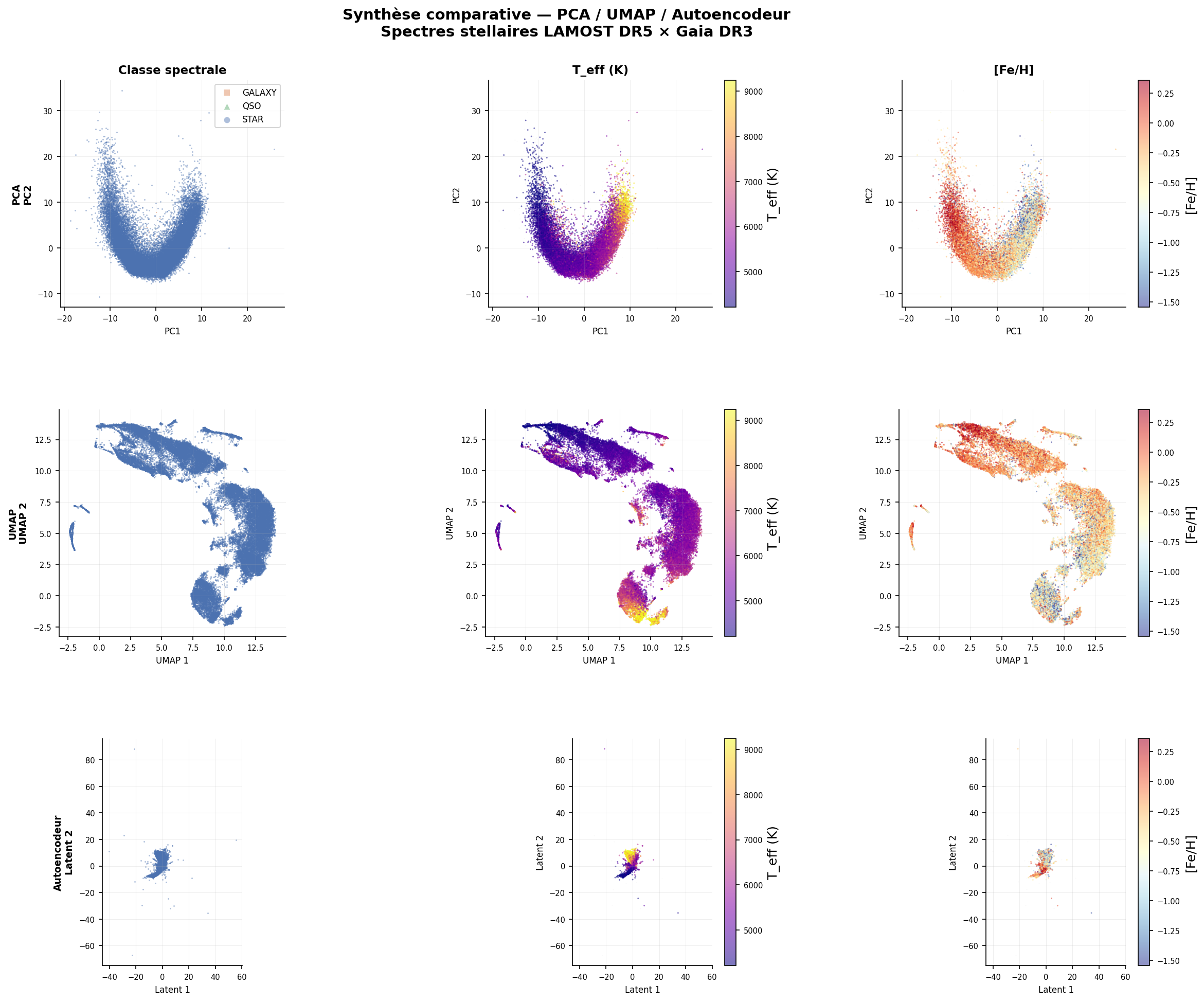
Synthesis: three latent spaces side by side — same data, different geometries
Physical structure captured by each method
All three methods capture the same underlying physical structure — but at different levels:
- PCA: Linear temperature gradient (ρ = +0.831) + partial metallicity separation
- UMAP: Non-linear Harvard sequence + dwarf/giant bifurcation + 20 HDBSCAN clusters
- t-SNE: Sharp A-F hotspot + compact G-K archipelago + isolated subgiant masses
- Autoencoder: Smooth continuous latent manifold enabling interpolation and generation
The convergence of all four methods on the same physical structure validates the 183 spectroscopic feature set as a physically meaningful representation of stellar spectra.