Guide: Spectrum Preprocessing
A raw spectrum from the LAMOST telescope is not directly usable for machine learning. Each spectrum encodes both the real physics of the star and instrumental artifacts: absolute-brightness variations between stars, photon noise, cosmic pixels, and differences in observing conditions. Preprocessing is the step that removes these biases while preserving the relevant physical information.
All preprocessing logic is encapsulated in SpectraPreprocessor. Orchestration is handled by spectra_manager.py, which applies the pipeline in parallel across the ~250,000 downloaded spectra.
Pipeline overview
The preprocessing pipeline proceeds through five sequential steps, from reading the raw FITS file to producing the 183-descriptor vector ready for training. Click each step to view the details.
Step 1 — Wavelength-grid reconstruction
The λ grid is not stored explicitly in LAMOST files: it must be reconstructed from the FITS header metadata. SpectraPreprocessor implements a robust fallback chain to handle the different conventions used across observing campaigns.
# Primary method — COEFF0 + COEFF1 (log-linear)
coeff0 = header['COEFF0']      # λ₀ of the first pixel (log10)
coeff1 = header['COEFF1']      # logarithmic step / pixel
n_pix  = flux.shape[0]         # 3921 channels
loglam  = coeff0 + np.arange(n_pix) * coeff1
wavelength = 10 ** loglam      # → Angstroms [3690 ... 9100]
Result: a vector of 3,921 wavelengths covering 3,690–9,100 Å, with a logarithmic step of Δlog(λ) ≈ 0.0001 (about ~1.36 Å/pixel at 5,500 Å).
Step 2 — Flux normalization
Stars have very different absolute brightnesses and distances — an A-type star at 500 pc may have an apparent flux 1,000 times higher than a nearby M dwarf. Without normalization, these magnitude differences dominate the features and hide spectral-type differences.
if median > 0: flux /= medianWhy median normalization is sufficient
Median normalization is deliberately simple: it answers the question “is this continuum above or below its average level?” without trying to model the continuum shape. This simplicity is a strength:
- Robustness — insensitive to emission lines and artifacts
- Reproducibility — one parameter, no arbitrary choices
- Fairness between descriptors — the StandardScaler applied afterward to the feature matrix completes the statistical normalization (mean 0, variance 1)
# Excerpt from SpectraPreprocessor.normalize_spectrum()
def normalize_spectrum(self, flux: np.ndarray) -> np.ndarray:
    """Normalize the flux by the median — robust to outliers."""
    positive_flux = flux[flux > 0]
    if len(positive_flux) == 0:
        return flux   # fully masked spectrum — return as is
    median_flux = np.median(positive_flux)
    if median_flux > 0:
        return flux / median_flux
    return flux
Step 3 — Continuum fitting for slopes
To extract local continuum slopes (Family 6 — ~65 descriptors), an additional sigma-clipping step is applied locally within each spectral window:
from astropy.stats import sigma_clip

def fit_local_slope(wavelength, flux, wl_min, wl_max, sigma=2.5):
    """
    Sigma-clipped linear fit of the local continuum.
    σ = 2.5 removes absorption lines without biasing the slope.
    """
    mask = (wavelength >= wl_min) & (wavelength <= wl_max)
    wl_local  = wavelength[mask]
    fl_local  = flux[mask]

    # Sigma-clipping — removes lines and artifacts
    clipped = sigma_clip(fl_local, sigma=sigma, maxiters=3)

    # Linear regression on the clean continuum
    coeffs = np.polyfit(wl_local[~clipped.mask], fl_local[~clipped.mask], deg=1)
    return coeffs[0]   # slope in flux/Å units
Five slopes are extracted: UV (3800–4200 Å), green visible (4500–5500 Å), red visible (5500–6500 Å), near IR (6500–7500 Å), and global slope (3800–7500 Å).
Local curvatures (Savitzky-Golay second derivative) follow the same principle:
from scipy.signal import savgol_filter

def compute_curvature(flux, wavelength, center_wl, window=50, polyorder=3):
    """Continuum curvature (second derivative) in Ångströms⁻²."""
    idx = np.argmin(np.abs(wavelength - center_wl))
    window_pts = min(window, idx, len(flux) - idx - 1)
    smooth = savgol_filter(flux, window_length=2*window_pts+1, polyorder=polyorder, deriv=2)
    return smooth[idx]
Step 4 — Quality filters
Two sequential filters ensure that only scientifically usable spectra enter the analysis:
Filter 1 — Signal-to-noise ratio
# SNR in the LAMOST red band (~6000–7000 Å)
mask_snr = catalog['snr_r'] > 10
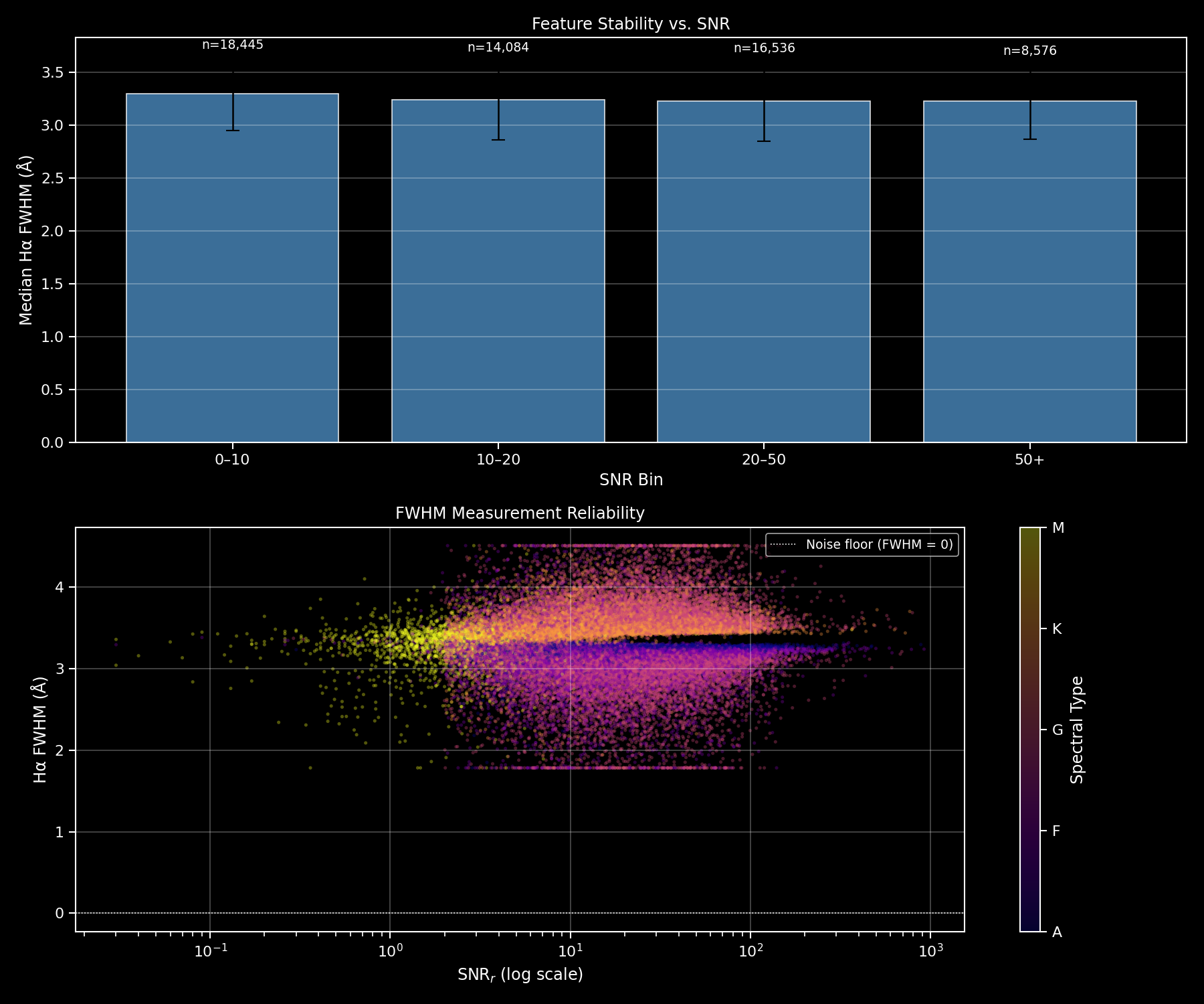
Justification: Below SNR = 10, the prominence of weak lines (Fe, Mg b) becomes comparable to the noise — the descriptors would be dominated by statistical artifacts. A threshold of 10 is the minimum for equivalent-width measurements to be reliable.
Filter 2 — RUWE astrometric quality (Gaia DR3)
# RUWE (Re-normalised Unit Weight Error) — Gaia astrometric-solution quality
mask_ruwe = catalog['ruwe'] < 1.4
Justification: RUWE > 1.4 indicates a faulty proper-motion solution — typically an unresolved binary star or a measurement artifact. Binary stars have composite spectra that blur the classification lines.
Filter impact
| Step | Spectra | Notes |
|---|---|---|
| Downloaded | ~250,000 | Raw FITS files |
| After SNR_r > 10 | ~180,000 | Usable spectra |
| After RUWE < 1.4 | ~150,000 | Reliable single sources |
| After Gaia 1″ cross-match | 43,019 | Final set with reference parameters |
Step 5 — Extraction of the 183 descriptors
Once the spectrum has been normalized and validated, FeatureEngineer.extract_features() computes the 183-physical-descriptor vector:
from src.pipeline.feature_engineering import FeatureEngineer

fe = FeatureEngineer()

# For each clean spectrum
vec = fe.extract_features(
    matched_lines,   # lines detected by peak_detector.py
    wavelength,      # reconstructed λ grid (3921 points)
    flux_norm,       # median-normalized flux
    invvar,          # inverse variance (pixel masking)
)
# vec: np.ndarray with shape (183,)
Measured processing throughput: ~340,000 spectra/hour (Ryzen 9 5950X, 32 threads, joblib parallelization).
Reference figures
Future improvement tracks
The current preprocessing is designed to be fast and robust on the ~250,000 available spectra. The project Roadmap includes:
- Polynomial continuum fitting — iterative method for stars with strong UV continuum
- Systematic denoising — Savitzky-Golay applied to the full spectrum before extracting weak lines
- Interstellar-extinction correction — A_G × R_V for strongly reddened stars
- Binary-spectrum processing — deconvolution of composite line profiles for the C19/C1/C12 clusters identified by HDBSCAN