First Run: From A to Z

Now that your environment is configured, we will run the complete pipeline through the main notebook: 00_master_pipeline.ipynb. This notebook orchestrates every step, from data selection to the generation of a session report.

Codespaces users

If you are using a Codespace, the environment is already ready. Open notebooks/ and launch 00_master_pipeline.ipynb. A small demonstration dataset may already be available depending on the Codespace configuration.

Checklist (30 seconds)

• You are running the notebook with the AstroSpectro (Py3.11) kernel, or an equivalent environment.
• Your .env file is configured if you use external credentials; see Gaia Connection.
• Locally, data/raw/ contains spectra. If not, complete Step 1 first.

Step 1: Acquire data (if needed)

If this is your very first local run, the data/raw/ directory will be empty:

1. Open the notebook notebooks/01_download_spectra.ipynb.
2. Use the interface below to start the download. For a quick test, select around 1000 spectra.

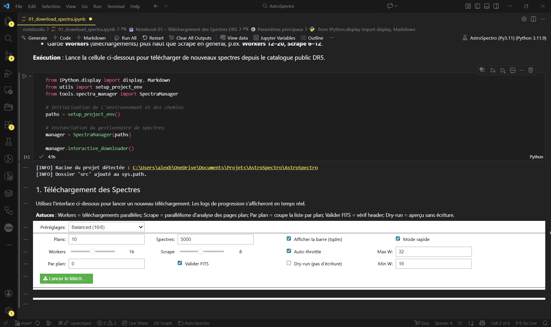
Figure 1: The interactive interface used to configure and start data acquisition.

Need the advanced options — workers, scrapes, tqdm, auto-throttle, FITS validation, or dry-run mode? They are documented in User Guides → Downloading Data.

Step 2: Run the complete pipeline

Once you have data:

1. Open the main notebook: notebooks/00_master_pipeline.ipynb.
2. Run all cells from top to bottom.

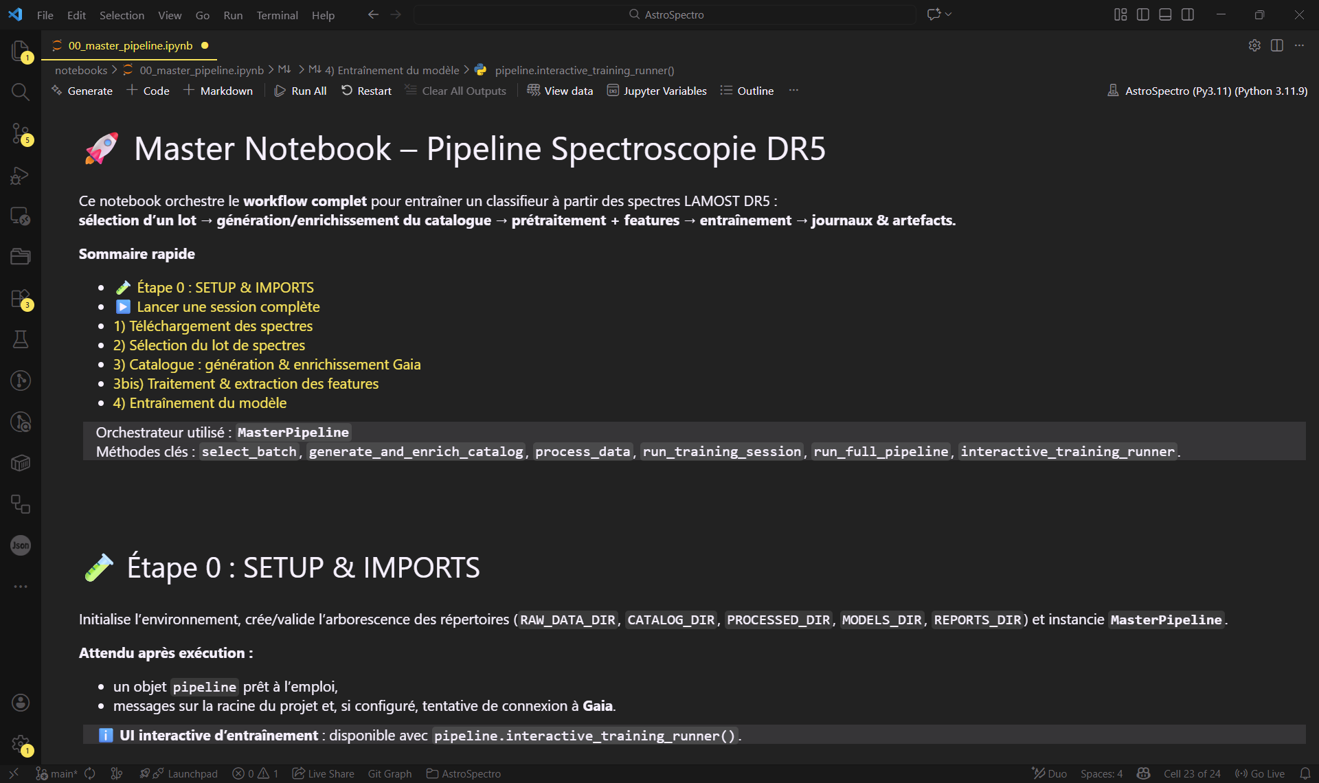
Figure 2: The main orchestrator (00_master_pipeline) ready to use.

The notebook runs the MasterPipeline sequentially:

• It initializes the environment, sets up access to Gaia, and creates or validates the required directory structure. The first connection may take a little while.
• Batch selection: simply define the number of desired spectra, for example batch_size=1000, and keep the default strategy, random.
• Local catalog generation for the selected batch.
• Processing & feature extraction, with several dozen possible features depending on the configuration.
• Training & evaluation through an interactive interface.

Training (recommended first run)

In the training interface, you can choose several models, such as XGBoost, RandomForest, SVM, ExtraTrees, KNN, MLP, and others, and adjust their hyperparameters.

Goal: validate that the full chain works, not optimize performance.

For a first run, keep things simple:

• For an initial run, we recommend XGBoost or RandomForest. They are fast and robust. You can explore the other models afterward.
• Keep the default values, or use a template/preset if one is available.
• Launch the batch/run.

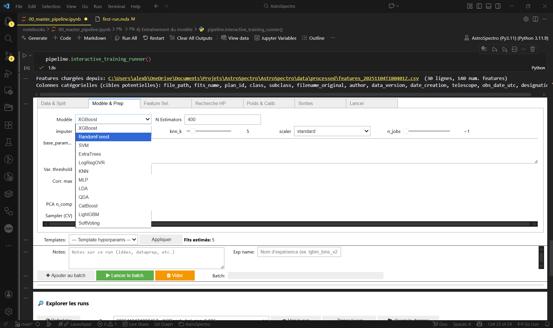
Figure 3: The control panel used to choose your model (XGBoost/RF) without touching the code.

The complete documentation on templates/presets, hyperparameter search, calibration, model choice, and related options is available in User Guides → Model Training.

Step 3: Review the results

At the end of the run, several artifacts are produced:

• A CSV file in data/processed/, containing features ready for analysis.
• A .pkl model in data/models/.
• A JSON session report in data/reports/, along with result-analysis figures such as feature_importance, roc, confusion_matrix, precision_recall, and others.

Congratulations

You have run the pipeline end to end and obtained your first classifications. You are ready to explore the project in more depth.

What next?

Related page	Relation
Understand the science	The astrophysical concepts behind the code: spectral classification, flux normalisation, equations
Become an expert	Configure workers, optimise downloads and build your own training presets