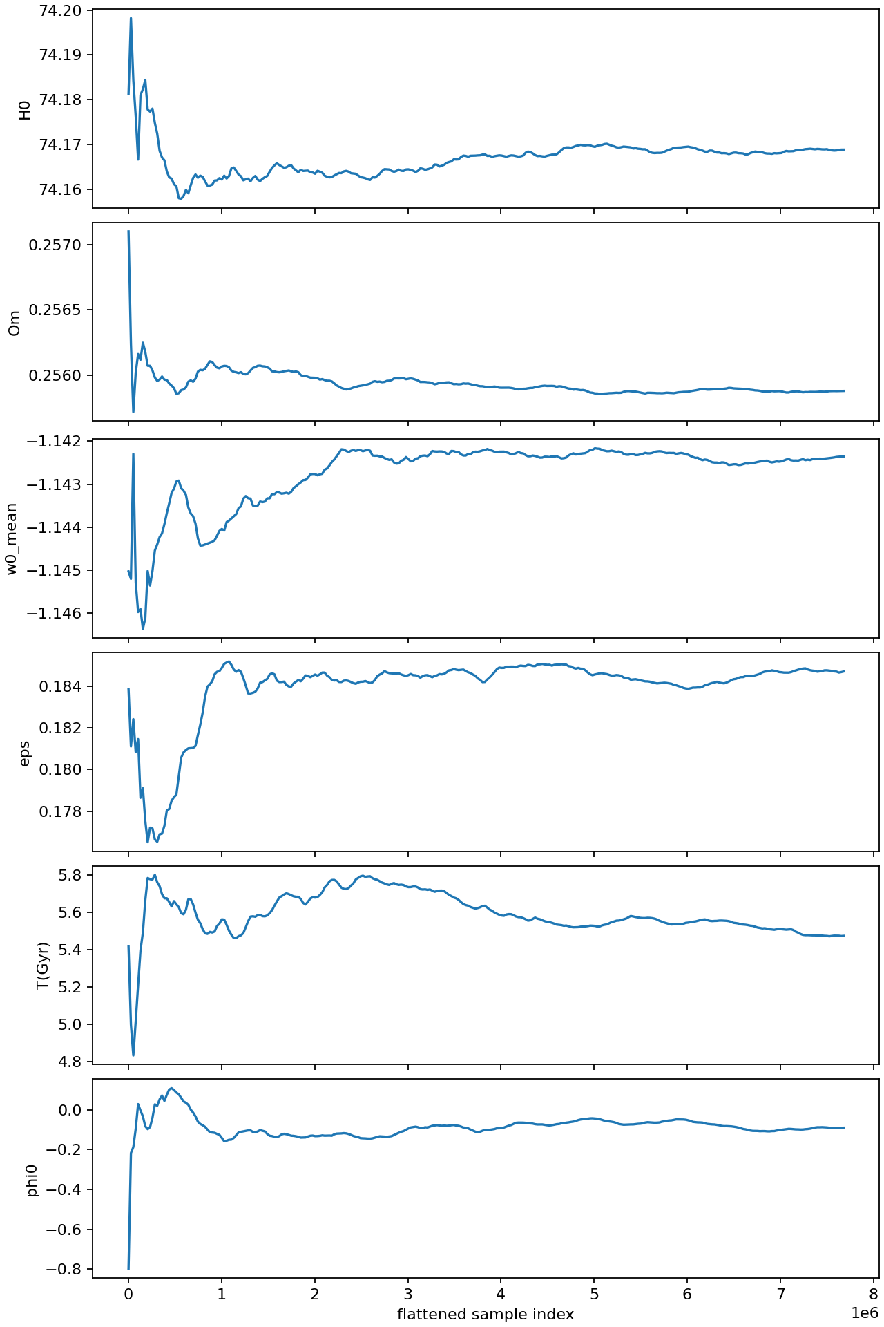
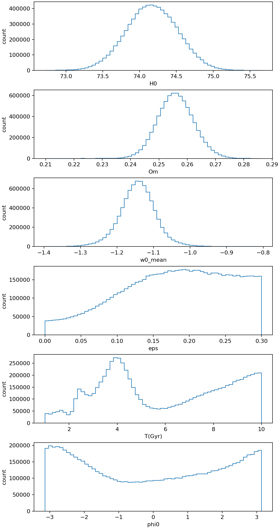
Convergence Diagnostics
This page reports the sampling diagnostics of the final Protocol 1b run (96 walkers × 100,000 steps) and states what they do and do not establish. The headline: the Ξosc chain meets the practical criterion N/50 > τmax, while T and φ₀ remain broad.
Key results
| Diagnostic | ΛCDM | CPL | Ξosc |
|---|---|---|---|
| Mean acceptance fraction | 0.715 | 0.594 | 0.180 |
| Largest τ | not in the exported files | not in the exported files | 1503.8 (parameter T) |
The exported run journal is truncated to its last 400 lines, which contain the autocorrelation times of Ξosc only. The project report quotes approximate values for the other two models, but no exported output file contains them, so they are not published here.
Autocorrelation times of Ξosc
emcee returns one integrated autocorrelation time per parameter (in steps). Those of Ξosc, computed on the full chain:
| Parameter | H₀ | Ωₘ | w₀,mean | ε | T | φ₀ |
|---|---|---|---|---|---|---|
| τ | 508.0 | 513.6 | 508.8 | 489.1 | 1503.8 | 1250.1 |
The cosmological parameters decorrelate in about 508 steps; the oscillation period T and phase φ₀ are markedly slower. That is expected from a periodic model: T and φ₀ are strongly coupled (see the diagonal bands in the T–φ₀ panel of the corner plot).
The practical criterion
The run uses the rule of thumb N/50 > τmax, where N is the number of steps per walker (convergence_flag in xi_cosmo.diagnostics, factor 50):
| Quantity | Value |
|---|---|
| N/50 | 2,000 |
| τmax (Ξosc) | 1503.8 |
| Criterion satisfied | yes |
For Ξosc N/50 exceeds τmax by a factor 1.33 — enough, but with little margin, for the slowest parameters.
The Ξosc acceptance fraction is low
Ξosc accepts 0.180 of proposals, against 0.715 for ΛCDM. A low value is typical when the posterior is narrow in some directions and bounded or multimodal in others; it is one reason the chain needs so many steps.
What these diagnostics do not test
| Not tested | Consequence |
|---|---|
| Multimodality / other starting regions | Walkers start from one fixed point (MCMC Setup); no multi-start or Gelman–Rubin comparison is implemented |
| Prior-boundary accumulation | A well-sampled posterior can still pile up against a bound (ε, T) — see Oscillation Diagnostic |
| Walker traces | Only the flattened chain is saved |
| ΛCDM and CPL τ | Not in the exported files |
Diagnostic figures from the saved chain
scripts/make_chain_diagnostics.py draws two lightweight figures from the flattened Ξosc chain. They are not trace plots.