Corner Plots
This page shows the posterior distributions as corner plots: one-dimensional marginals on the diagonal and two-dimensional contours below it. The reference figures are those of Protocol 1b (1,590 SNe + 13 BAO); the Pantheon-only Protocol 1 figures are included to show how the BAO data change the shapes.
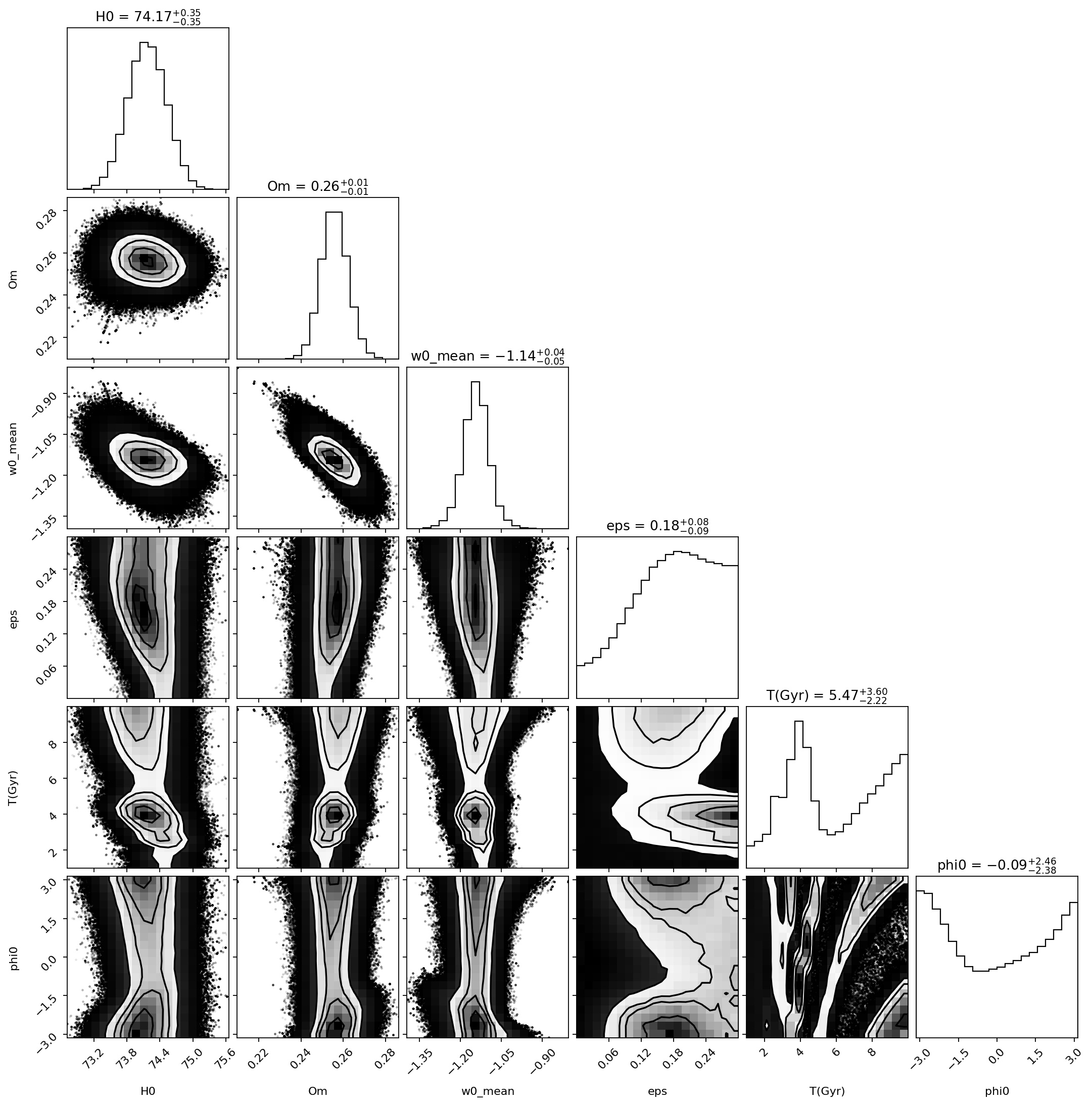
Protocol 1b — Pantheon+SH0ES + DESI DR2 BAO
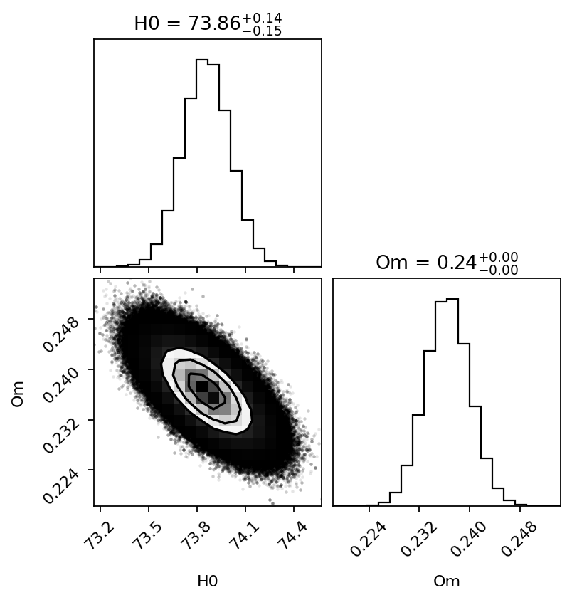
The corner plot of CPL for the final run is not part of the exported figure set, so none is shown here. The CPL constraints are in Parameter Constraints.
Reading the Ξosc plot
| Panel | What to look for | Reading |
|---|---|---|
| H₀, Ωₘ, w₀,mean marginals | single, near-Gaussian peaks | well constrained |
| Ωₘ – w₀,mean | tilted, elongated contour | anti-correlated: a more negative mean w goes with a smaller Ωₘ |
| ε marginal | density rises from ε = 0 and stays high up to the right-hand edge | the posterior is truncated by the prior upper bound (0 < ε < 0.3) |
| T marginal | a narrow peak at short T and a broad shoulder growing towards the upper edge | multi-featured, extends to the prior bound (1 < T < 10 Gyr) |
| φ₀ marginal | high at both ends, low in the middle | φ₀ is periodic, so the two ends are the same region: a mode near ±π |
| T – φ₀ | diagonal bands | T and φ₀ are degenerate (the same oscillation phase today can come from several (T, φ₀) pairs) |
The titles above each column quote the median and a symmetric ± at two decimals; for ε, T and φ₀ they hide the shape of the distributions, which is why the median is a poor summary for these three parameters.
Protocol 1 — Pantheon+SH0ES only (comparison)
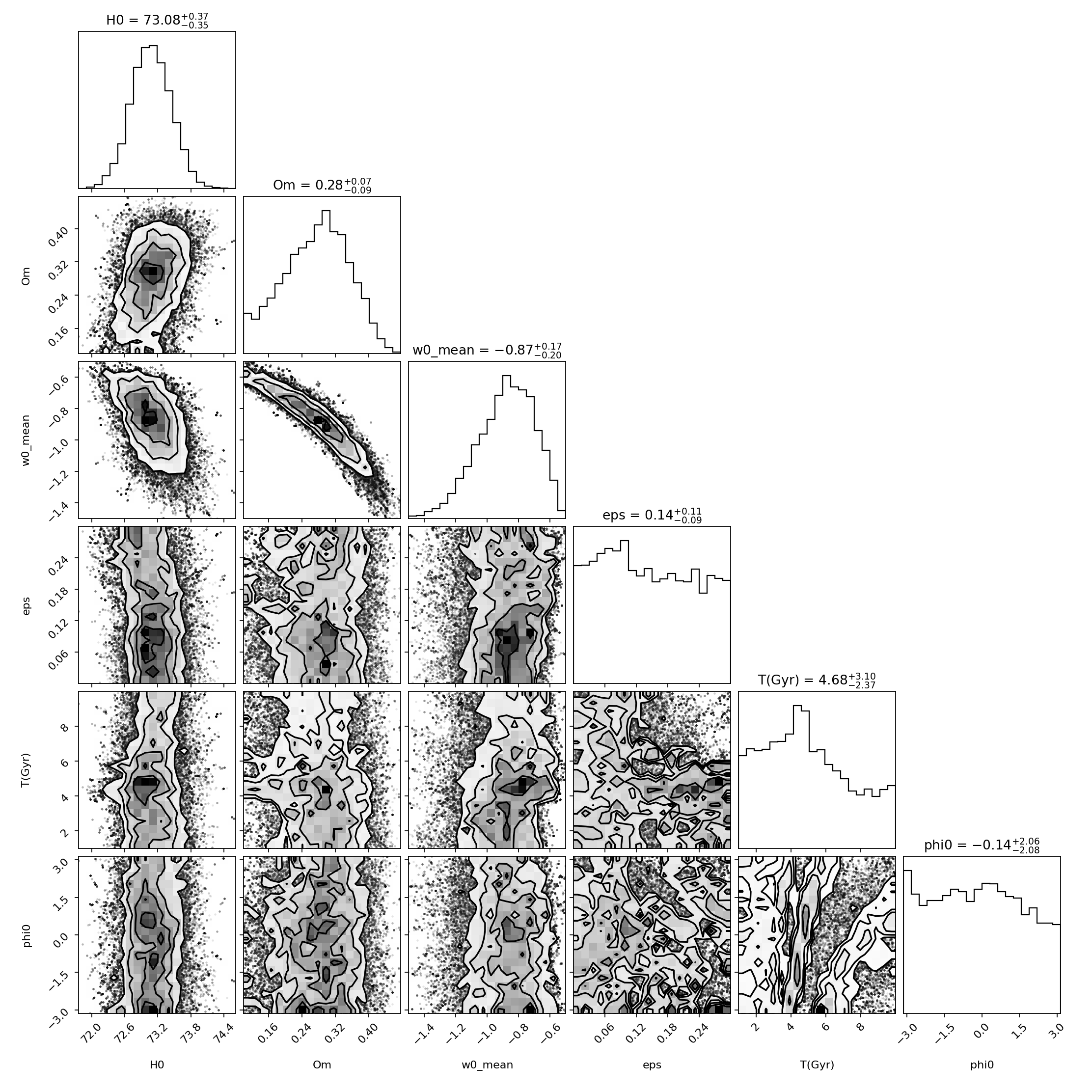
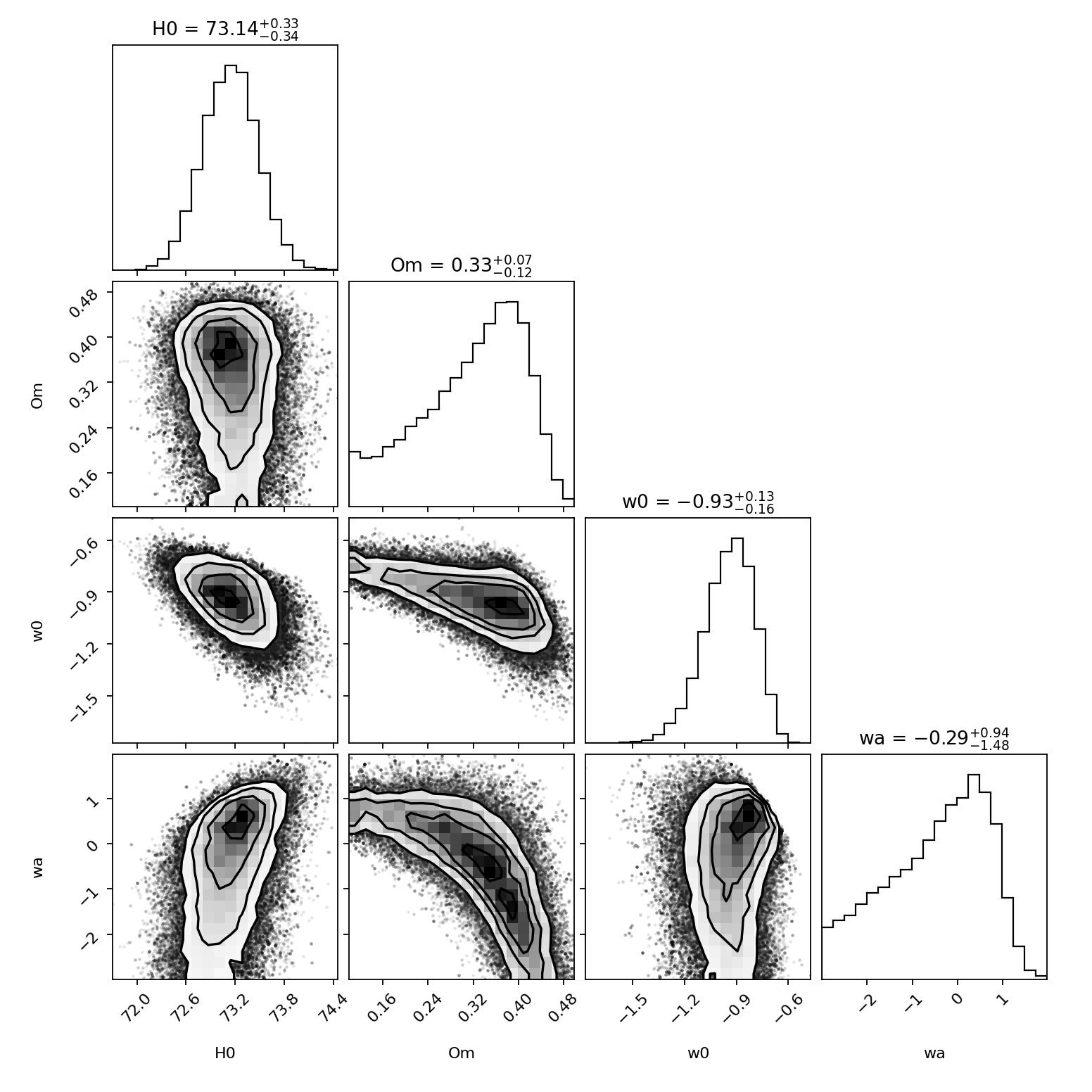
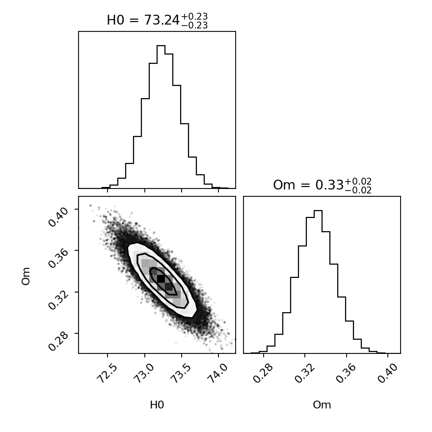
Protocol 1 used the supernovae alone (no BAO). The exported pack contains its three corner plots but no numerical summary and no record of its chain length, so no Protocol 1 number is quoted anywhere on this site and the figures are not a like-for-like comparison with the final run.